What is a GPU and Why Should You Care? (CPU vs. GPU, History, and the Compute Paradigm Shift)

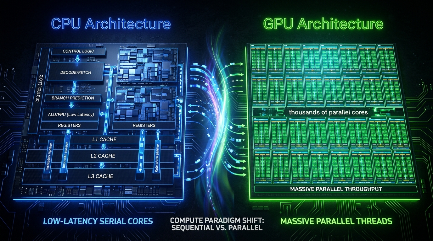
Series: Part 3 of GPU Architecture, Scale-Up Interconnects, and AI Datacenter Infrastructure Series | (Previous) From Transistors to Logic Gates: How Physics Turns into Math (CMOS, Adders, and ALUs) | (Next) Under the Silicon Hood: Core GPU Building Blocks and Stream Processors

Summary

For over four decades, the central dogma of microprocessor design was optimizing for single-thread latency: making an individual sequential thread execute as fast as humanly possible through deep out-of-order execution windows, multi-level speculative branch predictors, and massive on-die SRAM caches. But when deep neural networks emerged as the defining computing workload of the 21st century, single-thread latency became irrelevant. Training a 70-billion-parameter language model or rendering a photorealistic 4K video frame does not require executing one instruction in 0.2 nanoseconds; it requires executing tens of trillions of independent matrix multiplications per second.

In Part 3 of our GPU Architecture, Scale-Up Interconnects, and AI Datacenter Infrastructure Series, we deconstruct the foundational identity of the Graphics Processing Unit (GPU). We contrast the Ferrari vs. Cargo Ship architectural trade-off that separates CPUs from GPUs, explore the historical evolution from 1990s fixed-function 3D rasterization to programmable shaders and NVIDIA’s G80 unified architecture, examine how the release of CUDA in 2006 transformed graphics accelerators into general-purpose supercomputers, compare how silicon die area is budgeted between control logic and arithmetic logic units (ALUs), and analyze Amdahl’s Law versus Gustafson’s Law to understand why the AI revolution was born on parallel silicon.

Prior Reading Material

To trace how semiconductor hardware evolved from basic electronic switches to modern parallel architectures, explore these foundational articles:

From Transistors to Logic Gates: How Physics Turns into Math (CMOS, Adders, and ALUs) — Part 2: MOSFETs, CMOS static power cancellation, boolean logic, and ALU design.
From Sand to Silicon: The Semiconductor Fab, Wafers, Dies, and the Reticle Limit — Part 1: Czochralski ingots, ASML EUV lithography, and wafer defect density economics.
Basics of AI Inference: Compute vs Memory Bound — Operational intensity, memory bandwidth roofs, and FLOPS throughput boundaries.
vLLM on NVIDIA Vera Rubin NVL72: HBM4 Memory Subsystems and Petabyte Scale Serving — Petascale throughput scaling and ultra-high-bandwidth memory fabrics.

1. The Tale of Two Engines: Ferrari vs. Cargo Ship

To understand why a modern server pairs an AMD EPYC or Intel Xeon Central Processing Unit (CPU) with eight NVIDIA H100 or Blackwell B200 GPUs, consider a logistical analogy: delivering packages across a metropolis.

A CPU is a Formula 1 Ferrari. It carries a single passenger, accelerates to blistering speeds instantaneously, maneuvers through complex zig-zagging streets with hairpin turns, and delivers an urgent document from Point A to Point B with the absolute lowest possible latency. If your program consists of an operating system kernel handling page faults, interacting with network drivers, maintaining state machines, and executing branching if-else conditionals, the CPU is unmatched.

A GPU is an Oceanic Cargo Freighter. It accelerates slowly, has a wide turning radius, and cannot dart through narrow city alleys. If you task a cargo ship with delivering a single envelope across the harbor, it is embarrassingly inefficient. But if your task is to transport 24,000 shipping containers simultaneously across the Pacific Ocean, the cargo ship moves thousands of times more total mass per unit of fuel and time than an entire fleet of Ferraris.

flowchart TD
    classDef cpuStyle fill:#1e293b,stroke:#3b82f6,stroke-width:2px,color:#ffffff;

    subgraph CPU_Philosophy["CPU Silicon Philosophy: Minimize Latency for a Single Thread"]
        C1["High Clock Frequency (4.0 - 5.5 GHz)"]:::cpuStyle
        C2["Speculative Branch Prediction & Out-of-Order Execution"]:::cpuStyle
        C3["Gigantic Multi-Level Caches (L1, L2, 3D V-Cache L3)"]:::cpuStyle
        C4["Silicon Budget: ~70% Control Logic & Cache, ~30% ALU"]:::cpuStyle
        C1 --> C2 --> C3 --> C4
    end

flowchart TD
    classDef gpuStyle fill:#064e3b,stroke:#10b981,stroke-width:2px,color:#ffffff;

    subgraph GPU_Philosophy["GPU Silicon Philosophy: Maximize Aggregate Throughput"]
        G1["Moderate Clock Frequency (1.5 - 2.5 GHz)"]:::gpuStyle
        G2["Massive SIMD/SIMT Parallel Thread Execution"]:::gpuStyle
        G3["Hardware Thread Schedulers Hiding Memory Latency"]:::gpuStyle
        G4["Silicon Budget: ~80% Floating-Point ALUs, ~20% Cache/Control"]:::gpuStyle
        G1 --> G2 --> G3 --> G4
    end

Modern artificial intelligence workloads—such as multiplying weight matrices of dimensions $[4096 \times 14336] \times [14336 \times 4096]$ in a Transformer feed-forward layer—are embarrassingly parallel. Every element in the output matrix can be computed independently of every other element. There are no sequential dependencies or branch mispredictions to recover from; the only metric that matters is aggregate throughput (Floating-Point Operations Per Second, or FLOPS), not single-operation latency.

2. The Silicon Budget: How CPUs and GPUs Allocate Die Area

Why can’t a CPU simply execute parallel matrix multiplications as quickly as a GPU? The answer lies in the unforgiving physical constraints of the semiconductor die budget.

As explored in Part 1, the optical reticle limit caps monolithic chip sizes at approximately 858 mm². Within that finite two-dimensional silicon surface, chip architects must choose how to allocate every square millimeter of transistors.

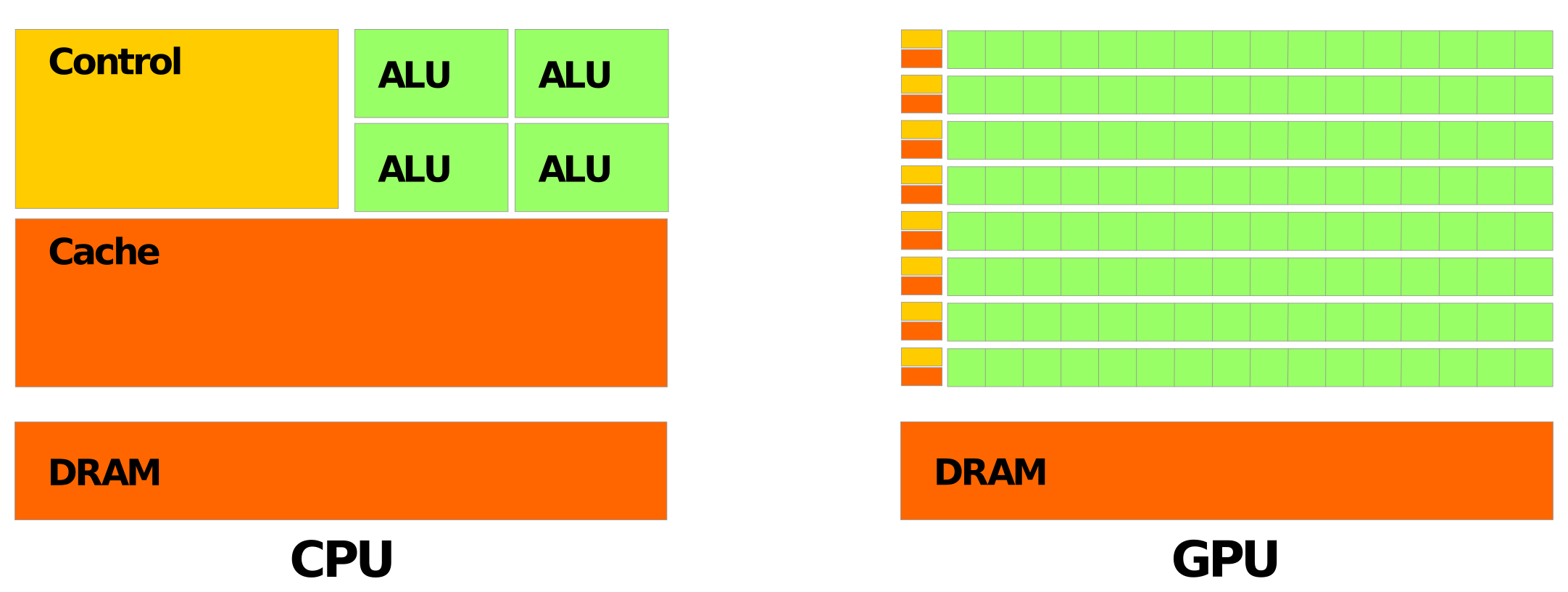CPU vs GPU Silicon Die Area Allocation Figure 1: Comparison of CPU vs. GPU silicon allocation. While CPUs prioritize low-latency serial execution with extensive control logic and multi-level caches, GPUs maximize arithmetic throughput by dedicating the vast majority of die area to thousands of parallel ALUs and massive register files. Source: Wikimedia Commons / NVIDIA CUDA Architecture Overview.

Where CPU Transistors Go

A high-performance modern CPU core spends only a small fraction of its area on basic arithmetic units. The majority of its silicon footprint is consumed by defensive circuitry designed to accelerate single-threaded execution and avoid memory stalls:

Branch Predictors & Trace Caches: Multi-megabyte predictors (such as TAGE) that guess the path of conditional jumps with 98%+ accuracy before instructions even decode.
Out-of-Order (OoO) Execution Windows & Reorder Buffers (ROB): Thousands of silicon tracks dedicated to analyzing instruction dependency graphs, dynamically reordering independent instructions, and renaming physical registers.
Deep Multi-Level SRAM Caches: L1 (32–64 KB per core), L2 (1–2 MB per core), and shared L3 (32–128+ MB) caches designed to keep the CPU execution units fed without stalling for the 50–80 ns penalty of main DDR5 DRAM access.

Where GPU Transistors Go

A GPU makes a radically different engineering wager. It abandons complex branch prediction and out-of-order execution entirely. Instead, a GPU assumes:

Instructions are executed in-order across wide SIMD (Single Instruction, Multiple Data) or SIMT (Single Instruction, Multiple Threads) vectors.
Memory latency is hidden by oversubscription: Rather than spending megabytes of silicon on huge L3 caches to keep one thread from stalling, a GPU maintains thousands of active thread contexts in massive register files. When Thread Warp 0 issues a high-latency load from global memory (taking 200–400 cycles), the hardware scheduler instantly switches to Thread Warp 1 in a single clock cycle, executing math while Warp 0 waits for data.
Maximized ALU Density: By stripping away speculative decode logic and branch prediction hardware, the GPU packs tens of thousands of floating-point adders, multipliers, and matrix Tensor Cores into the exact same silicon area.

3. Historical Odyssey: From Fixed-Function 3D to GPGPU

The modern AI GPU was not created overnight as a deep learning accelerator; it is the evolutionary culmination of a thirty-year race to render photorealistic three-dimensional computer graphics.

Figure 2: Thirty-year historical evolution of the GPU architecture. Tracing the path from fixed-function 3D rasterization silicon to programmable shaders, G80 unified compute cores, CUDA, the 2012 AlexNet deep learning breakthrough, and modern systolic Tensor Core superchips.

Era 1: Fixed-Function Silicon (1990s)

In the 1990s, companies like 3dfx (Voodoo Graphics), S3 Graphics, and early NVIDIA (NV1, RIVA 128, GeForce 256) built hardware dedicated to the fixed 3D graphics pipeline. Silicon circuits were hardwired to perform exactly four mathematical stages: vertex transform, triangle clipping, rasterization (converting triangles into pixel fragments), and Z-buffer depth testing. If a game developer wanted a custom lighting model or volumetric fog, the silicon could not accommodate it; the logic was physically etched into non-programmable CMOS gates.

Era 2: Programmable Shaders (2001–2005)

With Microsoft DirectX 8 and the NVIDIA GeForce 3, fixed-function silicon began to crack open. Developers gained the ability to run small assembly micro-programs called Vertex Shaders (transforming 3D geometry coordinates) and Pixel/Fragment Shaders (calculating the color and texture of each pixel).

However, silicon was still split into separate physical pools: a GPU might have 8 dedicated vertex units and 24 dedicated pixel units. If a scene had dense geometry but simple lighting, the pixel units sat completely idle while vertex units bottlenecked the frame rate.

Era 3: The Unified Shader Architecture & G80 (2006)

In November 2006, NVIDIA unveiled the GeForce 8800 GTX (G80 architecture), spearheaded by Chief Scientist Bill Dally and CEO Jensen Huang. G80 tore down the wall between vertex and pixel processors. It introduced identical, fully general-purpose programmable processor cores—termed Streaming Multiprocessors (SMs)—that could execute any arbitrary floating-point instruction stream. Whether calculating vertex positions, pixel colors, physics simulations, or acoustic ray tracing, the same arithmetic units processed the load.

Era 4: The Birth of CUDA and GPGPU (2006–2007)

With G80, NVIDIA launched CUDA (Compute Unified Device Architecture). Before CUDA, academic researchers attempting to run general-purpose mathematics (GPGPU) on graphics cards had to perform bizarre hacks: they cast scientific matrices as 2D textures, encoded numbers into RGB color channels, and disguised partial differential equation solvers as pixel fragment shaders.

CUDA exposed the underlying parallel silicon directly through standard C/C++ extensions (__global__, thread indexing threadIdx.x, and shared memory allocations), transforming the GPU into a massively parallel numerical supercomputer.

Era 5: The AlexNet Catalyst (2012)

While academic researchers had used CUDA for molecular dynamics and fluid mechanics, the seminal turning point occurred in 2012. Alex Krizhevsky, Ilya Sutskever, and Geoffrey Hinton entered AlexNet into the ImageNet Large Scale Visual Recognition Challenge. Written in hand-tuned CUDA code (cuda-convnet) running across two consumer NVIDIA GeForce GTX 580 gaming cards (each with 3GB of VRAM and 512 CUDA cores), AlexNet crushed traditional computer vision approaches by an unprecedented 10.8 percentage point margin. Deep learning had found its hardware engine.

4. Mathematical Laws of Parallelism: Amdahl vs. Gustafson

To understand why the computing world restructured itself around GPUs, we must examine two fundamental laws governing parallel processing speedup.

Amdahl’s Law: The Pessimistic Ceiling

Formulated by computer architect Gene Amdahl in 1967, Amdahl’s Law models the theoretical speedup of a program when executed across $N$ parallel execution units with a fixed problem size:

$$S_{\text{latency}}(N) = \frac{1}{(1 - p) + \frac{p}{N}}$$

Where:

$p$ is the proportion of the program that can be parallelized.
$1 - p$ is the strictly serial portion that must run sequentially.
$N$ is the number of parallel processor cores.

If a program has even a modest 5% serial portion ($1 - p = 0.05$), then even if you deploy an infinite number of GPU cores ($N \to \infty$), the maximum speedup is hard-capped at:

$$S_{\max} = \frac{1}{0.05} = 20\times$$

For decades, Amdahl’s Law led traditional computer scientists to argue that building chips with thousands of small cores was futile, because the sequential serial bottleneck would dominate runtime.

Gustafson’s Law: The AI Reality

In 1988, John Gustafson realized that computer scientists do not keep problem sizes fixed when given larger supercomputers. Instead, they expand the problem size to fully saturate the available hardware.

In the modern AI context, engineers do not use a cluster of 16,384 Blackwell GPUs to train a 10-million-parameter network in 5 seconds. They use that compute cluster to train a 1.8-trillion-parameter mixture-of-experts model on 15 trillion tokens:

$$S_{\text{throughput}}(N) = (1 - p) + p \cdot N = s + p \cdot N$$

Where $s$ is the serial execution time and $p$ is the parallel execution time on $N$ processors. When problem sizes scale, the parallel work grows quadratically or cubically ($O(D^2)$ to $O(D^3)$ in matrix dimensions), while serial overhead ($s$) remains roughly constant. The serial fraction shrinks to $0.0001%$, allowing near-linear scaling across tens of thousands of GPU cores.

5. Architectural Execution Comparison

To contrast how a CPU and a GPU process a data stream, let us trace how both architectures handle a vector addition operation: $C[i] = A[i] + B[i]$ for $i = 0 \dots 1,000,000$.

CPU Execution Flow (Serial with SIMD Extensions)

Thread fetch and branch predictor loads instruction.
Register renamer maps logical registers to physical architectural registers.
Out-of-order scheduler buffers up to 512 micro-ops in the Reorder Buffer.
AVX-512 SIMD unit computes 16 single-precision floats per clock cycle.
If data misses L1/L2 cache, the execution pipeline stalls or searches for independent out-of-order instructions to execute.

GPU Execution Flow (Massive Hardware Multithreading)

The developer launches a grid of 1,000,000 threads grouped into blocks of 256.
The GPU hardware thread scheduler assigns blocks to Streaming Multiprocessors (SMs).
The warp scheduler groups threads into lockstep clusters of 32 threads called Warps.
Every cycle, the warp scheduler broadcasts one instruction (FADD32) to 32 CUDA cores simultaneously.
If a warp stalls waiting for memory data from High Bandwidth Memory (HBM), the scheduler switches context in zero clock cycles to another ready warp. Millions of arithmetic operations interleave seamlessly, saturating the memory bus.

flowchart TD
    classDef stepStyle fill:#0f172a,stroke:#0284c7,stroke-width:2px,color:#ffffff;
    classDef schedStyle fill:#312e81,stroke:#6366f1,stroke-width:2px,color:#ffffff;
    classDef aluStyle fill:#064e3b,stroke:#10b981,stroke-width:2px,color:#ffffff;

    W1["Grid of 1,000,000 Independent Threads"]:::stepStyle
    W2["Hardware Block Distribution across Streaming Multiprocessors"]:::schedStyle
    W3["Warp Partitioning: 32 Threads per SIMT Warp"]:::schedStyle
    W4["Warp Scheduler selects ready warps with zero-cycle overhead"]:::schedStyle
    W5["Simultaneous execution across 128+ CUDA Cores per SM"]:::aluStyle

    W1 --> W2
    W2 --> W3
    W3 --> W4
    W4 --> W5

6. Hands-On Simulation: Latency vs. Throughput Benchmarking

To build concrete intuition for this computing paradigm shift, the following Python script models and simulates CPU serial execution, CPU multi-core vectorization, and GPU parallel execution. It measures wall-clock execution time, effective GFLOPS (Giga Floating-Point Operations Per Second), and arithmetic throughput as problem dimensions scale from $10^3$ to $10^7$ elements.

Click to expand runnable code script

"""
CPU vs GPU Architectural Execution Simulation.
Demonstrates latency-optimized serial execution vs throughput-optimized SIMD/GPU execution
across varying vector and matrix dimensions.
"""

import time
import numpy as np

def simulate_cpu_serial(size: int) -> tuple[float, float]:
    """Simulates a strictly serial, single-threaded execution loop (like a scalar CPU core)."""
    a = np.random.rand(size).astype(np.float32)
    b = np.random.rand(size).astype(np.float32)
    c = np.zeros(size, dtype=np.float32)
    
    start = time.perf_counter()
    # Python explicit loop emulating scalar CPU instructions without SIMD
    # (Testing on smaller slice to keep simulation responsive)
    eval_size = min(size, 200_000)
    for i in range(eval_size):
        c[i] = a[i] * b[i] + 0.5
    elapsed = time.perf_counter() - start
    
    # Scale elapsed time to full problem size
    normalized_time = elapsed * (size / eval_size)
    # 2 operations per element (multiply + add)
    gflops = (size * 2) / (normalized_time * 1e9)
    return normalized_time, gflops

def simulate_vectorized_cpu(size: int) -> tuple[float, float]:
    """Simulates an optimized CPU execution using AVX/SIMD vector registers and multi-threading."""
    a = np.random.rand(size).astype(np.float32)
    b = np.random.rand(size).astype(np.float32)
    
    # Warmup
    _ = a[:1000] * b[:1000] + 0.5
    
    start = time.perf_counter()
    c = a * b + 0.5
    elapsed = time.perf_counter() - start
    
    gflops = (size * 2) / (elapsed * 1e9)
    return elapsed, gflops

def simulate_gpu_parallel_model(size: int, num_cores: int = 16384, clock_ghz: float = 2.0) -> tuple[float, float]:
    """
    Simulates GPU execution using an analytical architectural model:
    - Fixed kernel launch and dispatch overhead (5 microseconds)
    - Memory bus latency hidden by warp oversubscription
    - Saturation across tens of thousands of parallel SIMT lanes
    """
    # 2 FLOPS per element (FMA: Fused Multiply-Add)
    total_flops = size * 2
    
    # Peak theoretical throughput of modeled GPU (e.g. NVIDIA H100 FP32 core array)
    peak_gflops = num_cores * clock_ghz * 2  # 2 FLOPS/cycle per core FMA
    
    # Memory bandwidth limit: 3.35 TB/s (H100 SXM5 HBM3)
    # Reading A (4 bytes), B (4 bytes), writing C (4 bytes) = 12 bytes/element
    memory_bytes = size * 12
    hbm_bandwidth_gb_s = 3350.0  # GB/s
    memory_transfer_time_s = memory_bytes / (hbm_bandwidth_gb_s * 1e9)
    
    # Compute time if perfectly parallelized
    compute_time_s = total_flops / (peak_gflops * 1e9)
    
    # Fixed PCIe / CUDA driver dispatch latency (~5 microseconds)
    driver_overhead_s = 5.0e-6
    
    # GPU execution time is bounded by the slower of compute vs memory (Roofline model) + overhead
    execution_time_s = max(compute_time_s, memory_transfer_time_s) + driver_overhead_s
    
    achieved_gflops = total_flops / (execution_time_s * 1e9)
    return execution_time_s, achieved_gflops

def main():
    print("=" * 78)
    print("CPU vs. GPU Execution Paradigm Benchmark Simulation")
    print("=" * 78)
    print(f"{'Data Size':<12} | {'Method':<20} | {'Time (ms)':<15} | {'Throughput (GFLOPS)':<20}")
    print("-" * 78)
    
    sizes = [10_000, 100_000, 1_000_000, 10_000_000]
    
    for size in sizes:
        # 1. Scalar CPU Simulation
        t_scalar, g_scalar = simulate_cpu_serial(size)
        print(f"{size:<12} | {'CPU Scalar':<20} | {t_scalar * 1e3:>12.3f} ms | {g_scalar:>17.3f}")
        
        # 2. Vectorized CPU (SIMD)
        t_simd, g_simd = simulate_vectorized_cpu(size)
        print(f"{size:<12} | {'CPU SIMD (AVX)':<20} | {t_simd * 1e3:>12.3f} ms | {g_simd:>17.3f}")
        
        # 3. Modeled High-Throughput GPU
        t_gpu, g_gpu = simulate_gpu_parallel_model(size)
        print(f"{size:<12} | {'GPU SIMT Model':<20} | {t_gpu * 1e3:>12.3f} ms | {g_gpu:>17.3f}")
        print("-" * 78)

if __name__ == "__main__":
    main()

What’s Next in the Series?

Now that we have established why the computing world pivoted from latency-optimized CPUs to throughput-optimized parallel silicon, we are ready to open the silicon package and inspect the physical hardware layout.

In Part 4: Under the Silicon Hood: Core GPU Building Blocks and Stream Processors, we will examine the physical floorplan of modern GPUs: Graphics Processing Clusters (GPCs), Texture Processing Clusters (TPCs), Streaming Multiprocessors (SMs), FP32/INT32 execution datapaths, and how instruction caches and register files are physically partitioned across the die.