
TPUs vs. NPUs vs. GPUs: The Architecture of Specialized AI Accelerators (Google TPU v1–v6e, Edge Neural Engines, Groq LPU, and Cerebras)
Beyond the GPU: An architectural deep-dive into Google TPUs, Edge NPUs, and Spatial ASICs—contrasting systolic arrays, deterministic SRAM, and sub-5W silicon.
GPU & AI Hardware Architecture Series: ← What is a GPU and Why Should You Care? (CPU vs. GPU, History, and the Compute Paradigm Shift) (Previous) | Under the Silicon Hood: Core GPU Building Blocks and Stream Processors (Next) →
Summary
The modern artificial intelligence boom was ignited on general-purpose GPUs, but running frontier deep learning exclusively on graphics architectures introduces structural trade-offs. While GPUs dedicate substantial die area to general-purpose SIMT schedulers, dynamic warp dispatchers, and multi-level cache hierarchies, neural network compute is overwhelmingly dominated by a single mathematical primitive: matrix multiplication ($D = A \times B + C$).
This specialization gap sparked the domain-specific accelerator revolution. In this deep dive, we explore the architectural spectrum beyond the GPU:
- Google TPUs (v1 through Trillium v6e): How 2D systolic arrays eliminate the Von Neumann register energy wall by rhythmically streaming data across processing elements with stationary weight accumulation and direct Inter-Chip Interconnect (ICI) optical fabrics.
- Edge NPUs (Apple Neural Engine & Qualcomm Hexagon): How mobile SoCs deliver 45–75 TOPS within strict sub-5-watt thermal envelopes by leveraging unified memory architectures (UMA), fused activation pipelines, and integer quantization.
- Spatial ASICs (Groq LPU, Cerebras WSE-3, and Tenstorrent): How replacing dynamic hardware scheduling and external HBM with software-scheduled deterministic SRAM fabrics achieves sub-millisecond time-to-first-token and 800+ tokens-per-second generation speeds.
Prior Reading Material
To build a solid foundation on how silicon logic gates, physical transistor budgets, and GPU pipelines operate, we recommend reading through these prerequisites:
- From Sand to Silicon: The Semiconductor Fab, Wafers, Dies, and the Reticle Limit — The photolithographic limits, wafer defect economics, and physical boundaries shaping modern processors.
- From Transistors to Logic Gates: How Physics Turns into Math (CMOS, Adders, and ALUs) — How MOSFETs, FinFETs, and CMOS logic gates are assembled into digital arithmetic logic units.
- What is a GPU and Why Should You Care? (CPU vs. GPU, History, and the Compute Paradigm Shift) — The foundational CPU vs. GPU paradigm shift, Amdahl’s Law, and how GPUs allocate 80% of their die to parallel compute.
- Google Gemini 3.8 Flash: High-Throughput Multimodal Speed and Efficiency — Real-world examination of sub-second streaming inference served natively on Google TPU v6e Trillium clusters.
- Silicon at the Edge: NVIDIA Jetson Thor Architecture & Isaac ROS Acceleration — Heterogeneous edge architectures combining high-performance GPU cores with low-power deep learning accelerators (DLAs).
1. Beyond the Cargo Ship: The Accelerator Spectrum
In yesterday’s deep dive on What is a GPU and Why Should You Care?, we established the classic computer architecture analogy:
- The CPU is a Formula 1 Racer: Built for blistering single-thread speed. It navigates complex, unpredictable decision branches with massive instruction windows, out-of-order execution logic, and multi-megabyte SRAM caches, dedicating approximately 70% of its silicon die area purely to control flow and latency mitigation.
- The GPU is an Oceanic Cargo Freighter: Built for aggregate throughput. It sacrifices single-thread agility to pack thousands of floating-point ALUs and wide register files into roughly 80% of its die area, moving 24,000 shipping containers simultaneously by hiding high-latency memory transactions behind massive multithreaded thread oversubscription.
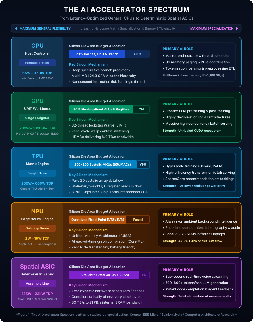 Figure 1: Architectural comparison of the modern AI computing spectrum from latency-oriented CPUs to spatial deterministic ASICs. Source: IEEE Micro / SemiAnalysis / Computer Architecture Research.
However, as powerful as the GPU freighter is, it was engineered as a programmable parallel computer. It retains hardware thread schedulers, warp instruction caches, texture pipelines, and complex register crossbars.
When you know in advance that over 95% of your computing workload consists solely of General Matrix Multiplies (GEMMs), general-purpose graphics silicon carries an unavoidable energy and silicon tax. This realization split the hardware landscape into five distinct architectural paradigms:
- CPUs (Host Controllers): Unmatched sequential control, memory mapping, and complex system orchestration.
- GPUs (SIMT Workhorses): Unrivaled programmable parallelism, deep software tooling (CUDA), and supreme flexibility across evolving research architectures.
- TPUs (Datacenter Systolic Engines): Custom silicon optimized purely for deterministic 2D matrix multiplication at hyperscale datacenter efficiency.
- NPUs (Edge Neural Processors): Co-processors integrated directly into mobile and laptop SoCs, designed to deliver high inference throughput within a strict 2-watt to 15-watt thermal envelope.
- Spatial ASICs (Deterministic Dataflow Fabrics): Processors like the Groq LPU and Cerebras Wafer-Scale Engine that abandon off-chip memory and runtime scheduling entirely, routing data across massive arrays of on-chip SRAM in compile-time lockstep.
2. Google TPUs: Conquering the Von Neumann Energy Wall
When Google engineers began analyzing their datacenter workloads in 2013, they calculated that if every Android user utilized voice search for just three minutes per day, Google would need to double its entire global datacenter footprint simply to run the acoustic neural networks. General-purpose CPUs and GPUs were too power-hungry and expensive to scale linearly with global query volume.
This prompted the secretive development of the Tensor Processing Unit (TPU), deployed into Google datacenters in 2015.
flowchart TD
    A["Von Neumann Bottleneck: Every multiply requires reading 2 operands from Register SRAM"]:::redStyle
    --> B["The Energy Wall: Register File reads consume 10x more energy than the math itself"]:::redStyle
    --> C["The Systolic Solution: 2D Grid of Processing Elements (Kung & Leiserson)"]:::blueStyle
    --> D["Weights remain stationary in local cell registers"]:::blueStyle
    --> E["Activations stream horizontally, partial sums accumulate vertically"]:::blueStyle
    --> F["65,536 Multiply-Accumulates per cycle with ZERO register reads during traversal"]:::blueStyle

    classDef redStyle fill:#450a0a,stroke:#ef4444,stroke-width:2px,color:#fecaca;
    classDef blueStyle fill:#0c4a6e,stroke:#38bdf8,stroke-width:2px,color:#e0f2fe;
The Physics of the Systolic Array
The fundamental genius of the TPU lies in the Systolic Array, a computing concept first formalized by H.T. Kung and Charles Leiserson in 1978.
In a conventional Von Neumann CPU or GPU datapath, executing a multiply-accumulate operation requires:
- Fetching operand $A$ from an on-chip register file.
- Fetching operand $B$ from an on-chip register file.
- Performing the multiplication $A \times B$ in an ALU.
- Writing the partial sum back to a register.
In deep-submicron semiconductor nodes, shuttling bits across metal wires and reading SRAM register cells consumes up to ten times more picojoules of energy than the mathematical calculation itself. When multiplying a 4096-wide matrix, a standard processor expends 90% of its thermal budget simply moving numbers back and forth to registers.
A systolic array completely bypasses this register traffic by mimicking the rhythmic pumping of the human heart (hence systolic):
- Inside a 2D matrix of Processing Elements (PEs), model weights are loaded once and held stationary inside local registers.
- Input activation tokens are fed into the left edge of the grid, pulsing horizontally across the array one cell per clock cycle.
- As an activation passes through a cell, it is multiplied by the stationary weight and added to the partial sum arriving from the cell directly above it.
- The accumulating partial sums flow vertically downward, emerging from the bottom of the grid as the final completed matrix output.
Because data flows directly from neighbor to neighbor across short, dedicated silicon wires, the TPU performs tens of thousands of multiplications per clock cycle with near-zero register memory reads.
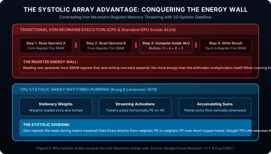 Figure 2: Why 2D systolic arrays conquer the Von Neumann register energy wall. Source: Google Cloud Research / H.T. Kung (CMU).
Generational Odyssey: From TPU v1 to Trillium v6e
Google’s TPU architecture evolved from an auxiliary PCIe coprocessor into the backbone of world-scale foundation model training:
- TPU v1 (2015): A pure 28nm inference engine connected over PCIe Gen3. It featured a single 256x256 8-bit Matrix Multiply Unit (MXU) delivering 92 TOPs. It lacked floating-point support and had no direct networking.
- TPU v2 & v3 (2017–2018): Introduced the 16-bit Brain Floating Point (BF16) format that preserved the dynamic range of FP32 while slashing memory footprint in half. TPU v3 added liquid cooling and integrated direct Inter-Chip Interconnects (ICI), allowing chips to link into high-speed 2D/3D torus topologies without passing through expensive datacenter Ethernet switches.
- TPU v4 & v5p (2021–2023): Integrated Optical Circuit Switches (OCS) that dynamically reconfigure the optical fiber topology between racks in milliseconds. TPU v5p scaled to 8,960 chips per pod with 4,800 Gbps ICI bandwidth per chip.
- TPU v6e “Trillium” (2024–Present): Google’s 6th-generation workhorse, optimized specifically for modern transformer serving and agentic models like Gemini 3.8 Flash:
- Dual 256 × 256 MXUs: Doubling the systolic dimensions of the v5 generation to execute 65,536 MACs per cycle.
- Peak Throughput: Delivers 918 TFLOPs of BF16 and 1,836 TOPs of INT8 per chip.
- Memory Subsystem: 32 GB of High Bandwidth Memory (HBM) delivering 1,638 GB/s (~1.6 TB/s) bandwidth.
- SparseCores: Dedicated on-chip hardware accelerators designed specifically to handle irregular memory gather-scatter operations for embedding-heavy recommendation engines.
- Inter-Chip Interconnect (ICI): 4 ICI ports providing 3,200 Gbps aggregate bandwidth arranged in a 2D Torus.
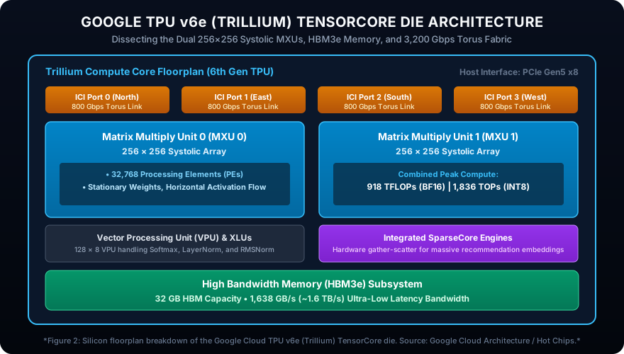 Figure 3: Silicon floorplan breakdown of the Google Cloud TPU v6e (Trillium) TensorCore die. Source: Google Cloud Architecture / Hot Chips.
3. Edge NPUs: Ambient AI Inside a 5-Watt Envelope
While datacenters optimize for raw matrix throughput per megawatt, edge devices—smartphones, laptops, AR glasses, and embedded robots—operate under brutal physical constraints: a sealed aluminum chassis, fanless passive cooling, and a 3,000 to 5,000 mAh battery.
Running continuous inference on a laptop GPU draws 30W to 80W of power, draining the battery in under ninety minutes while scorching the user’s lap. This necessitated the creation of the Neural Processing Unit (NPU).
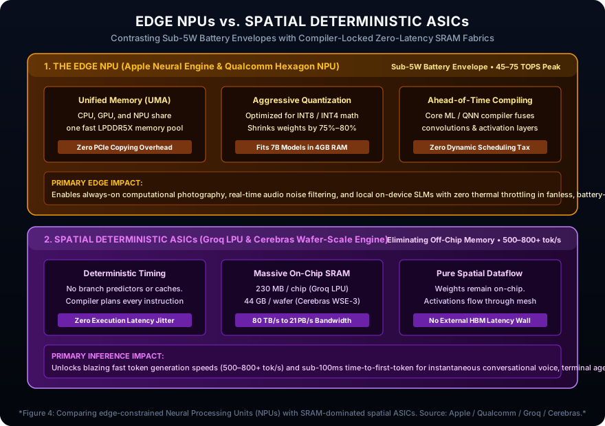 Figure 4: Comparing edge-constrained Neural Processing Units (NPUs) with SRAM-dominated spatial ASICs (Groq LPU and Cerebras WSE). Source: Apple Platform Architecture / Qualcomm Snapdragon / Hot Chips.
The Three Tenets of Edge NPU Design
Unlike datacenter processors that prioritize high-precision training and massive memory buses, modern NPUs—such as the Apple Neural Engine (ANE), Qualcomm Hexagon NPU, and Intel AI Boost / AMD Ryzen AI—adhere to three uncompromising principles:
flowchart TD
    N1["1. Unified Memory Architecture (UMA)"]:::amberStyle
    --> N2["Zero CPU-to-GPU PCIe memory copying; shared high-bandwidth LPDDR5X"]:::amberStyle
    --> N3["2. Aggressive Integer Quantization (INT8 & INT4)"]:::amberStyle
    --> N4["Slashing memory footprint by 75% and doubling arithmetic density"]:::amberStyle
    --> N5["3. Ahead-of-Time Graph Compilation (Core ML / QNN)"]:::amberStyle
    --> N6["Hardware scheduler completely omitted; OS schedules static execution"]:::amberStyle

    classDef amberStyle fill:#78350f,stroke:#fbbf24,stroke-width:2px,color:#fef3c7;
1. Unified Memory Architecture (UMA)
In a traditional desktop with a discrete GPU, running inference requires copying input audio, camera frames, and model weights over the PCIe bus from system RAM to dedicated VRAM. This bus transfer introduces millisecond latency spikes and consumes significant battery wattage.
In modern edge SoCs (such as the Apple M4 or Snapdragon X Elite), the CPU, GPU, and NPU sit on the same silicon substrate and share a single pool of unified memory (delivering 100 to 400+ GB/s bandwidth). When the camera captures a 4K frame, the NPU processes the tensor directly in place without a single byte of memory duplication.
2. The Dominance of Integer Quantization
Floating-point arithmetic (FP32 or FP16) requires complex exponent alignment logic, sign management, and large silicon multipliers. By quantizing models to INT8 (8-bit integer) or INT4 (4-bit integer):
- Silicon area per multiplier shrinks by up to 80%.
- Memory bus transfers consume one-quarter the power of FP16.
- An edge device can fit a 3B or 7B parameter foundation model entirely within 4 GB of RAM, executing local on-device generation at 30+ tokens per second while consuming less than 4 watts.
3. Ahead-of-Time Graph Compilation
Unlike a GPU that dynamically schedules thread warps at runtime using complex silicon dispatch logic, an NPU relies on an ahead-of-time compiler (like Apple’s Core ML compiler or Qualcomm’s AI Engine Direct SDK). The compiler inspects the computational graph, fuses layers together (e.g., merging convolution, batch normalization, and ReLU into a single clock cycle), and sequences the exact flow of data through fixed-function matrix arrays.
Because the hardware doesn’t need to make runtime scheduling decisions, the silicon die can strip away instruction decoders and dynamic caches, maximizing the physical area allocated directly to matrix multipliers.
The TOPS Metric vs. Real-World Bandwidth Reality
In marketing materials, NPU capabilities are almost universally summarized in TOPS (Trillion Operations Per Second):
- Apple M4 Neural Engine: 38 TOPS
- Qualcomm Snapdragon X Elite Hexagon: 45 TOPS
- AMD Ryzen AI 300 series: 50 TOPS
- Intel Lunar Lake NPU: 48 TOPS
However, high TOPS numbers can be deceptive. A chip capable of 50 TOPS can only achieve that speed if its memory subsystem can supply weights and activations fast enough to prevent arithmetic starvation.
In generative LLM decoding, where a single token is generated per forward pass, throughput is bounded by memory bandwidth rather than raw TOPS. An NPU with 45 TOPS operating on a 136 GB/s LPDDR5X bus will generate tokens at roughly the same speed as a GPU sharing the same bus. The NPU’s true advantage is energy efficiency: it generates those tokens consuming 5 watts instead of 45 watts.
4. Spatial ASICs: Determinism, SRAM, and the Abolition of Memory Latency
While Google TPUs optimized datacenter matrix multiplication using HBM and systolic arrays, a radical class of hardware startups asked an even more provocative question:
“What if we completely eliminate external DRAM, HBM, and hardware schedulers entirely?”
This philosophy created Spatial Deterministic ASICs, led by Groq, Cerebras, and Tenstorrent.
Groq LPU: “Determinism is Speed”
Conventional GPUs and CPUs suffer from latency jitter. Cache misses, dynamic thread branch divergence, PCIe bus contention, and memory controller arbitration cause execution times to fluctuate unpredictably. When serving large language models across distributed clusters, the slowest chip in the collective communication step (AllReduce) bottlenecks every other processor.
The Groq Language Processing Unit (LPU) solves this by adopting an uncompromising design philosophy:
- Zero Dynamic Hardware Schedulers: The chip has no hardware instruction decoders, no out-of-order execution buffers, and no branch predictors.
- 230 MB of Pure On-Chip SRAM: Instead of connecting to slow, high-latency off-chip HBM, every Groq chip packs 230 megabytes of ultra-dense on-chip SRAM delivering 80 Terabytes per second of internal memory bandwidth.
- Compiler-Locked Determinism: The Groq compiler plans the exact physical trajectory of every electron. It knows precisely which clock cycle an activation will arrive at a given arithmetic functional unit. Because every operation executes in lockstep time-slots, there are zero memory stalls, zero pipeline bubbles, and zero synchronization barriers.
By streaming model activations across an interconnected mesh of LPUs, Groq systems achieve real-time generation speeds exceeding 500 to 800 tokens per second on Llama and Mixtral models—enabling conversational voice and instant code generation that feels instantaneous to human perception.
Cerebras WSE-3: The Wafer-Scale Supercomputer
If Groq’s answer to the memory wall was networking hundreds of SRAM-centric chips, Cerebras Systems took the most physically audacious route in semiconductor history: they refused to cut the silicon wafer at all.
In standard semiconductor manufacturing, a 300mm silicon wafer is diced into hundreds of individual rectangular dies (such as an 800 mm² NVIDIA H100). Cerebras prints an entire single processor across the entire 300mm wafer:
- Die Area: 46,225 mm² of contiguous silicon (compared to ~858 mm² for a reticle-limited GPU).
- Transistor Budget: 4 trillion transistors on TSMC 5nm.
- Compute Cores: 900,000 AI-optimized cores on a single piece of silicon.
- On-Chip SRAM: An unprecedented 44 Gigabytes of distributed on-chip SRAM.
- Internal Interconnect Bandwidth: A staggering 21 Petabytes per second.
By keeping entire multi-billion parameter neural networks resident inside a unified 44GB on-chip SRAM fabric, activations flow through a 2D mesh network without ever crossing a solder ball, substrate interposer, or PCIe cable.
5. Architectural Comparison Matrix
To synthesize how these processors contrast against one another, the table below breaks down the physical specifications, memory topologies, and target deployment tiers across the computing spectrum:
| Architectural Metric | Modern CPU (x86 / ARM) | Modern GPU (NVIDIA Blackwell) | Datacenter TPU (Google Trillium v6e) | Edge NPU (Snapdragon / Apple ANE) | Spatial ASIC (Groq LPU) |
|---|---|---|---|---|---|
| Primary Design Paradigm | Latency-oriented scalar / out-of-order | Throughput-oriented SIMT massively parallel | Systolic 2D Matrix Array engine | Energy-constrained SoC co-processor | Spatial deterministic dataflow |
| Die Area Allocation | ~70% Caches, Branch logic, OoO | ~80% ALUs & wide Register Files | Predominantly 256x256 Matrix Multiply Units | Fused fixed-point INT8/INT4 matrix blocks | Distributed SRAM & direct functional units |
| Typical Arithmetic Peak | 2–5 TFLOPs FP32 | 4,500 TFLOPs FP4 / 2,250 TFLOPs FP8 | 918 TFLOPs BF16 / 1,836 TOPs INT8 | 45–75 TOPs INT8 | ~750 TOPs INT8 |
| Memory Architecture | Off-chip DDR5 DRAM (50–100 GB/s) | HBM3e 3D Stacked (8.0 TB/s) | HBM3e 3D Stacked (1.6 TB/s) | Shared LPDDR5X UMA (100–400 GB/s) | 230 MB pure on-chip SRAM (80 TB/s) |
| Interconnect Fabric | PCIe Gen5 / UPI / Infinity Fabric | NVLink 5 (1.8 TB/s per GPU) | ICI 2D Torus (3,200 Gbps aggregate) | On-die AXI / Fabric crossbar | Direct chip-to-chip copper mesh |
| Typical Thermal Envelope | 65W – 350W | 700W – 1,000W+ | 250W – 600W | 2W – 15W (Sub-5W ambient) | 185W – 300W |
| Primary Software Stack | C++, Rust, Python, OpenMP | CUDA, Triton, TensorRT, PyTorch | JAX, XLA, PyTorch / XLA, TensorFlow | Core ML, ONNX, Qualcomm QNN | Groq Compiler (deterministic IR) |
| Ideal Operational Tier | Complex system orchestration, ETL | Frontier LLM pretraining & multimodal | Hyperscale training, batch inference | Always-on ambient assistants, cameras | Real-time conversational streaming |
6. Hands-On: Simulating the Architectural Spectrum
To experience the performance and energy trade-offs between CPUs, GPUs, TPUs, NPUs, and Spatial ASICs firsthand, we developed a zero-dependency Python simulator.
The script models the operational dynamics of multiplying a 4096-token sequence across a transformer projection layer: calculating arithmetic clock cycles, off-chip memory traffic, register file energy consumption, and thermal power draw.
Click to expand runnable code script: AI Silicon Paradigm Benchmark Simulator
#!/usr/bin/env python3
"""
AI Silicon Paradigm Benchmark Simulator
Simulates execution cycles, memory bandwidth utilization, energy consumption,
and throughput across CPU, GPU, TPU, Edge NPU, and Spatial ASIC architectures.
"""

from dataclasses import dataclass
from typing import Dict, List


@dataclass
class HardwareSpec:
    name: str
    paradigm: str
    peak_ops_per_sec: float     # In Operations/sec (FLOPs or INT-OPs)
    memory_bandwidth_gb_s: float # Off-chip memory bandwidth in GB/s
    on_chip_sram_mb: float       # On-chip SRAM in MB
    register_energy_factor: float# Relative energy spent on register/memory movement (1.0 = Von Neumann baseline)
    tdp_watts: float             # Thermal Design Power in Watts


def run_benchmark(batch_size: int, seq_len: int, d_model: int, d_ff: int):
    # Total multiply-accumulate operations for GEMM: [B * S, d_model] x [d_model, d_ff]
    # Each MAC counts as 2 floating/integer operations
    total_tokens = batch_size * seq_len
    total_ops = 2.0 * total_tokens * d_model * d_ff
    weight_bytes = d_model * d_ff * 2  # 2 bytes per parameter (FP16 / BF16)
    activation_bytes = total_tokens * d_model * 2

    print("=" * 80)
    print(f"  AI ACCELERATOR BENCHMARK: Transformer GEMM Projection Layer")
    print(f"  Tokens: {total_tokens:,} | d_model: {d_model} | d_ff: {d_ff}")
    print(f"  Total Math Operations: {total_ops / 1e9:.2f} GigaOps")
    print(f"  Weight Footprint: {weight_bytes / 1e6:.2f} MB")
    print("=" * 80)

    hardware_fleet: List[HardwareSpec] = [
        HardwareSpec("Server CPU (x86_64)", "Scalar + AVX-512", 4.0e12, 100.0, 64.0, 1.00, 250.0),
        HardwareSpec("Flagship GPU (H100)", "SIMT + Tensor Cores", 1.0e15, 3350.0, 50.0, 0.45, 700.0),
        HardwareSpec("Google TPU v6e", "2D Systolic MXU", 9.18e14, 1638.0, 32.0, 0.12, 450.0),
        HardwareSpec("Edge NPU (Mobile)", "Quantized Matrix Unit", 4.5e13, 136.0, 16.0, 0.15, 5.0),
        HardwareSpec("Spatial ASIC (Groq)", "Deterministic SRAM Fabric", 7.5e14, 80000.0, 230.0, 0.05, 200.0),
    ]

    results = []

    for hw in hardware_fleet:
        # Time required by raw compute ceiling (seconds)
        t_compute = total_ops / hw.peak_ops_per_sec

        # Time required to fetch weights & activations (seconds)
        if hw.on_chip_sram_mb >= (weight_bytes / 1e6):
            # Weights fit entirely on-chip in SRAM!
            bytes_transferred = activation_bytes
            t_memory = bytes_transferred / (hw.memory_bandwidth_gb_s * 1e9)
            sram_hit = True
        else:
            bytes_transferred = weight_bytes + activation_bytes
            t_memory = bytes_transferred / (hw.memory_bandwidth_gb_s * 1e9)
            sram_hit = False

        # Actual execution time bounded by the bottleneck (compute-bound vs memory-bound)
        t_exec = max(t_compute, t_memory)
        throughput_tokens_sec = total_tokens / t_exec

        # Energy calculation: Power * Time * Register movement efficiency
        energy_joules = hw.tdp_watts * t_exec * hw.register_energy_factor
        efficiency_tokens_per_joule = total_tokens / energy_joules if energy_joules > 0 else 0

        bottleneck = "Compute" if t_compute >= t_memory else "Memory BW"
        if sram_hit:
            bottleneck += " (SRAM Resident)"

        results.append({
            "name": hw.name,
            "paradigm": hw.paradigm,
            "latency_ms": t_exec * 1000.0,
            "tokens_sec": throughput_tokens_sec,
            "energy_j": energy_joules,
            "eff_tok_j": efficiency_tokens_per_joule,
            "bottleneck": bottleneck
        })

    # Display comparison results
    header = f"{'Processor':<22} | {'Latency':<9} | {'Throughput':<14} | {'Energy':<10} | {'Efficiency':<12} | {'Bottleneck'}"
    print(header)
    print("-" * len(header))
    for r in results:
        print(f"{r['name']:<22} | {r['latency_ms']:>6.2f} ms | {r['tokens_sec']:>10.0f} tok/s | {r['energy_j']:>7.3f} J | {r['eff_tok_j']:>8.1f} tok/J | {r['bottleneck']}")

    print("\n" + "=" * 80)
    print("  ARCHITECTURAL TAKEAWAYS:")
    print("  1. The CPU is throttled by memory bandwidth and small ALU count (100 GB/s bus).")
    print("  2. The GPU delivers massive raw throughput but draws 700W during execution.")
    print("  3. The TPU's systolic dataflow slashes register movement energy by ~88% over Von Neumann.")
    print("  4. The Edge NPU generates tokens with stunning energy efficiency (sub-5W envelope).")
    print("  5. The Spatial ASIC fits weights in 80 TB/s SRAM, obliterating memory wait states.")
    print("=" * 80)


if __name__ == "__main__":
    # Simulate a forward pass projection layer: Batch 1, Sequence 4096, d_model=4096, d_ff=14336
    run_benchmark(batch_size=1, seq_len=4096, d_model=4096, d_ff=14336)
Conclusion & Forward Teaser
The story of artificial intelligence hardware is not a zero-sum battle between CPUs and GPUs. It is an evolutionary continuum of specialization:
- When your software demands dynamic branching and operating system coordination, the CPU is indispensable.
- When research architectures are mutating monthly and require extreme programmable flexibility, the GPU remains the reigning sovereign.
- When datacenter foundation models scale into trillion-parameter cluster training, the TPU’s systolic simplicity and optical torus interconnects redefine cost economics.
- When ambient intelligence must operate continuously inside pocket-sized batteries, the Edge NPU delivers intelligence without heat.
- When millisecond conversational streaming requires eliminating off-chip memory bottlenecks, Spatial ASICs prove that compiler determinism is speed.
In the upcoming chapters of our hardware odyssey, we will return under the hood of modern silicon to inspect the granular anatomy of the GPU itself: how streaming multiprocessors schedule threads, how registers manage warp occupancy, and how advanced chiplet packaging overcomes the optical limits of physics.
GPU & AI Hardware Architecture Series: ← What is a GPU and Why Should You Care? (CPU vs. GPU, History, and the Compute Paradigm Shift) (Previous) | Under the Silicon Hood: Core GPU Building Blocks and Stream Processors (Next) →