
Wan 2.1: Open-Weight Video Diffusion, 3D VAE Latent Compression, and Consumer GPU Inference
Demystifying Wan 2.1: open-weight Diffusion Transformers, 3D causal VAE latent compression, Flow Matching math, and consumer GPU inference.
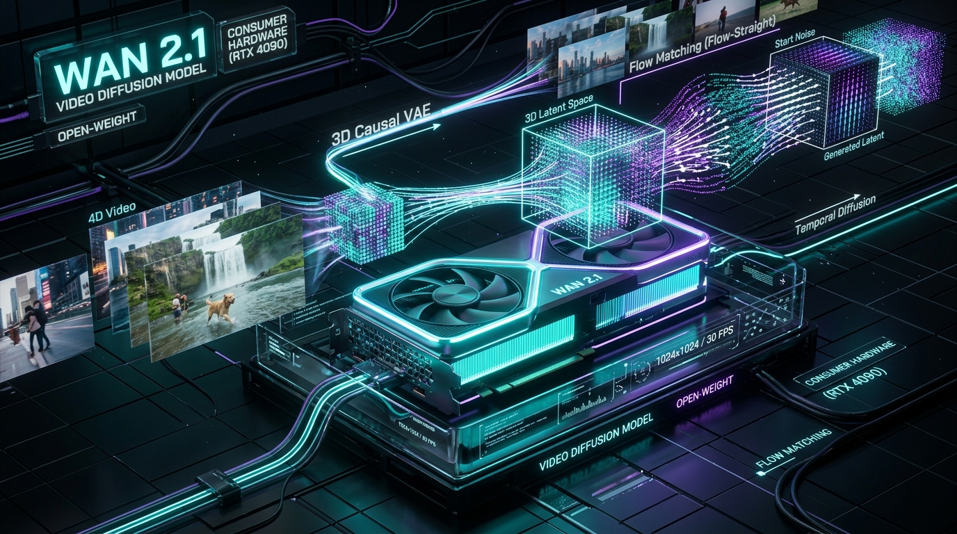
Series: ← ByteDance Seedance: Universal @-Reference Control, Multi-Modal Inputs, and Dual-Branch Audio-Video Diffusion (Previous)
Prior Reading Material
Before exploring Wan 2.1 and self-hosted open-weight video diffusion architectures, review these foundational deep-dives across our blog:
- Part 2: ByteDance Seedance: Universal @-Reference Control, Multi-Modal Inputs, and Dual-Branch Audio-Video Diffusion — Multi-Modality Diffusion Transformers (MMDiT), 3D MM-RoPE, and joint acoustic-visual flow matching.
- Part 1: Inside Higgsfield AI: Video Diffusion Architectures, Free Developer APIs, and the Generative Media Revolution — Spatiotemporal Video Diffusion Transformers (VDT), 3D camera trajectory splines, and developer API workflows.
- Part 2: Inside NVIDIA Cosmos: World Foundation Models for Physical Commonsense & Video Trajectories — Spatiotemporal latent tokenizers ($8 \times 8 \times 8$ compression) and score-matching diffusion architectures.
- What is an Omni Model? Architectural Taxonomy Across Qwen, Gemini, and NVIDIA Cosmos — Early-fusion continuous token spaces vs. late-fusion multimodal adapters across vision, audio, and physical worlds.
Official Model Card & Open-Weight Release Summary
While proprietary video generation platforms (such as Higgsfield, Kling, and Runway) operate behind gated cloud APIs, Wan 2.1—developed by Alibaba’s Tongyi Lab—represents a monumental breakthrough for the open-source AI community. Wan 2.1 is an open-weight video foundation suite built from the ground up to bring cinema-grade text-to-video (T2V) and image-to-video (I2V) generation directly onto consumer desktop hardware.
Featuring both a nimble 1.3B parameter model (fitting within ~8.2 GB of VRAM) and a flagship 14B parameter model capable of native 720p/1080p generation, Wan 2.1 combines a Flow Matching Diffusion Transformer (DiT) backbone with a novel 3D Causal Variational Autoencoder (Wan-VAE).
| Specification Field | Technical Detail & Official References |
|---|---|
| Developer / Lab | Alibaba Tongyi Lab (Wan Team) |
| Official Hugging Face Hub | Hugging Face: Wan-Video/Wan2.1 Collection |
| Technical Report | Wan 2.1: Open and Advanced Large-Scale Video Generative Models |
| Model Variants | Wan2.1-T2V-1.3B, Wan2.1-T2V-14B, Wan2.1-I2V-14B-720P, Wan2.1-I2V-14B-480P |
| Generative Paradigm | Flow Matching on 3D Spatiotemporal Latent Manifolds |
| Compression Architecture | 3D Causal VAE (Wan-VAE) with $8 \times 8 \times 4$ compression ratio ($x, y, t$) |
| Text Encoder | Multilingual Google T5-XXL / UMT5 cross-attention conditioning |
| Consumer Hardware Target | NVIDIA GeForce RTX 3060 / 4060 (1.3B) & RTX 4090 / 5090 (14B via FP8 / CPU Offloading) |
| Ecosystem Support | Diffusers, ComfyUI native nodes, FlashAttention-2, and TensorRT-LLM |
| Licensing | Apache 2.0 (Open-Weight & Commercial Permissive) |
1. The High-Speed Train & Video Compression Analogy
To understand how Wan 2.1 runs 1080p video diffusion on consumer GPUs without crashing into Out-Of-Memory (OOM) errors, consider how high-speed freight trains operate.
flowchart TD
    subgraph WanTrainPipeline["Wan 2.1 Causal Compression & Diffusion Pipeline"]
        direction TB
        F1["1. Raw Video Input: 81 Frames at 720p (~675 MB Uncompressed Pixels)"]
        V1["2. 3D Causal VAE: 8x Spatial & 4x Temporal Causal Compression"]
        V2["3. Compressed 3D Latent Volume: 21 x 90 x 160 x 16 (~9.6 MB Latent Grid)"]
        D1["4. Flow Matching DiT: Straight-Path Velocity Vector Field v_theta"]
        O1["5. FP8 Quantized Weights: Flagship 14B Model Fits in 16 GB Consumer VRAM"]
        O2["6. Causal Decoder Unpacks 4D Latents into 720p/1080p Cinema Video"]
    end

    F1 --> V1
    V1 --> V2
    V2 --> D1
    D1 --> O1
    O1 --> O2

    style WanTrainPipeline fill:#0d2b45,stroke:#00e5ff,stroke-width:2px,color:#ffffff
    style F1 fill:#0f172a,stroke:#00e5ff,stroke-width:1px,color:#ffffff
    style V1 fill:#0f172a,stroke:#10b981,stroke-width:1px,color:#ffffff
    style V2 fill:#0f172a,stroke:#10b981,stroke-width:1px,color:#ffffff
    style D1 fill:#0f172a,stroke:#8b5cf6,stroke-width:1px,color:#ffffff
    style O1 fill:#0f172a,stroke:#ec4899,stroke-width:1px,color:#ffffff
    style O2 fill:#0f172a,stroke:#34d399,stroke-width:1px,color:#ffffff
The Freight Bottleneck
If you attempt to transport bulk steel across country highways using millions of individual pickup trucks, traffic grinds to a halt. In deep learning, uncompressed video is that gridlock: a 5-second 720p video clip at 16 frames per second contains over $81 \times 720 \times 1280 \times 3$ values—amounting to roughly 224 million individual float numbers. Attempting to run multi-head self-attention directly across raw pixel tensors would require terabytes of GPU memory.
The 3D Causal VAE Solution
Wan 2.1 uses a specialized high-speed freight container: Wan-VAE.
- Spatial Compression ($8 \times 8$): Compresses pixel patches into compact 16-channel feature vectors.
- Temporal Compression ($4 \times$): Compresses every 4 consecutive temporal frames into a single latent timestep while preserving past causal context.
- The Result: The raw 224M pixel volume is reduced to an ultra-dense latent grid of $21 \times 90 \times 160 \times 16$. This $70\times$ volume compression allows consumer GPU memory buses to transfer and denoise entire cinematic sequences with sub-second step latency.
2. Architectural Blueprint: 3D Causal VAE and Flow Matching DiT
The complete end-to-end inference flow of Wan 2.1 is illustrated below:
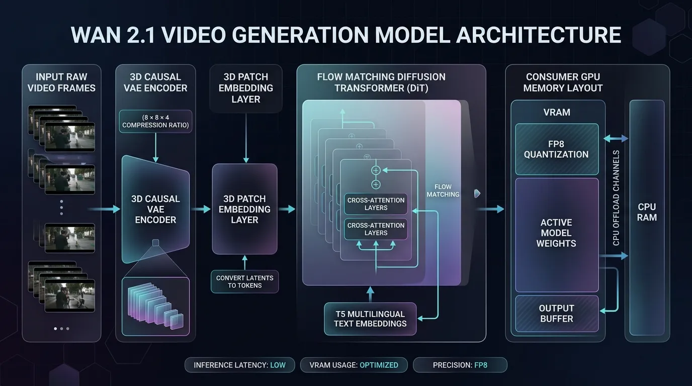
flowchart TD
    subgraph WanPipeline["Wan 2.1 End-to-End Generative Pipeline"]
        direction TB
        P1["Text Prompt / Image Anchor Input"]
        P2["T5-XXL Multilingual Tokenizer & Cross-Attention Text Matrix"]
        P3["Gaussian Noise Initialization: Z_1 ~ N(0, I) in Latent Space"]
        P4["Flow Matching DiT Backbone: Linear Vector Field Integration (t=1 -> t=0)"]
        P5["FP8 Quantized Transformer Blocks with Layer-Wise Offloading"]
        P6["3D Causal VAE Decoder: 8x8x4 Reconstruction to 720p/1080p MP4"]
    end

    P1 --> P2
    P2 --> P3
    P3 --> P4
    P4 --> P5
    P5 --> P6

    style WanPipeline fill:#0d2b45,stroke:#00e5ff,stroke-width:2px,color:#ffffff
    style P1 fill:#0f172a,stroke:#00e5ff,stroke-width:1px,color:#ffffff
    style P2 fill:#0f172a,stroke:#10b981,stroke-width:1px,color:#ffffff
    style P3 fill:#0f172a,stroke:#8b5cf6,stroke-width:1px,color:#ffffff
    style P4 fill:#0f172a,stroke:#ec4899,stroke-width:1px,color:#ffffff
    style P5 fill:#0f172a,stroke:#34d399,stroke-width:1px,color:#ffffff
    style P6 fill:#0f172a,stroke:#38bdf8,stroke-width:1px,color:#ffffff
Why 3D Causal VAE Matters
Most 2D image VAEs (such as those in Stable Diffusion XL or FLUX) are applied frame-by-frame. When decoding a sequence of independently encoded frames, slight floating-point variations cause severe temporal flickering and background jitter.
Standard 3D VAEs solve flickering by applying 3D convolutions across both space and time. However, non-causal 3D convolutions peek into future frames, making continuous video streaming and arbitrary length extension impossible.
Wan-VAE enforces strict temporal causality:
- The convolution receptive field for frame $t$ depends strictly on current and preceding frames ($\tau \le t$).
- The first frame is encoded identically to a still 2D image, ensuring zero degradation for Image-to-Video (I2V) conditioning tasks.
- Subsequent frames attend backward in time, eliminating temporal seams when stitching video chunks together.
3. Mathematical Foundations: Flow Matching vs. Traditional Diffusion
Earlier diffusion models (like DDPM and DDIM) rely on curved stochastic differential equations (SDEs) or curved probability flow ODEs. Denoising along curved trajectories requires 30 to 50 sequential steps to reach high visual fidelity.
Wan 2.1 replaces curved diffusion trajectories with Continuous Normalizing Flows via Flow Matching.
1. Straight-Path Velocity Interpolation
In Flow Matching, the generative trajectory between standard Gaussian noise $\mathbf{x}_1 \sim \mathcal{N}(0, \mathbf{I})$ and the true video data distribution $\mathbf{x}_0$ is defined as a straight linear interpolation:
$$\mathbf{x}_t = (1 - t) \mathbf{x}_0 + t \mathbf{x}_1, \quad t \in [0, 1]$$
The instantaneous time derivative (the true ground-truth velocity vector) is simply the constant difference between noise and data:
$$\frac{d\mathbf{x}_t}{dt} = \mathbf{x}_1 - \mathbf{x}_0$$
2. The Flow Matching Objective
The Diffusion Transformer $\mathbf{v}_\theta(\mathbf{x}_t, t, \mathbf{c})$ is trained to predict this straight velocity vector field conditioned on text embeddings $\mathbf{c}$:
$$\mathcal{L}{\text{FlowMatching}} = \mathbb{E}{t \sim \mathcal{U}[0, 1], ; \mathbf{x}_0, ; \mathbf{x}1} \left[ \left| \mathbf{v}\theta(\mathbf{x}_t, t, \mathbf{c}) - (\mathbf{x}_1 - \mathbf{x}_0) \right|^2 \right]$$
3. Inference Euler Integration
Because the vector field learned by Flow Matching is significantly straighter than curved DDPM probability flows, numerical integration during inference converges in as few as 15 to 25 steps using simple forward Euler integration:
$$\mathbf{x}_{t - \Delta t} = \mathbf{x}t - \Delta t \cdot \mathbf{v}\theta(\mathbf{x}_t, t, \mathbf{c})$$
This algorithmic linearity drastically reduces GPU floating-point operations (FLOPs), enabling real-time generation speeds on desktop hardware.
4. Running Wan 2.1 on Consumer Hardware: Optimization Strategies
Generating high-definition video requires careful memory orchestration. Here is how Wan 2.1 achieves consumer desktop execution:
flowchart TD
    subgraph MemoryOrchestration["Consumer GPU VRAM Optimization Techniques"]
        direction TB
        M1["Model Weight Precision: FP8 / INT4 Quantization (50% VRAM Cut)"]
        M2["Text Encoder Offloading: T5-XXL Execution -> System RAM Transfer"]
        M3["Spatially Tiled VAE Decoding: Splitting Latents into Overlapping Tiles"]
        M4["FlashAttention-2 & Memory-Efficient Kernel Fusion"]
    end

    M1 --> M2
    M2 --> M3
    M3 --> M4

    style MemoryOrchestration fill:#0d2b45,stroke:#00e5ff,stroke-width:2px,color:#ffffff
    style M1 fill:#0f172a,stroke:#00e5ff,stroke-width:1px,color:#ffffff
    style M2 fill:#0f172a,stroke:#10b981,stroke-width:1px,color:#ffffff
    style M3 fill:#0f172a,stroke:#8b5cf6,stroke-width:1px,color:#ffffff
    style M4 fill:#0f172a,stroke:#34d399,stroke-width:1px,color:#ffffff
1. FP8 Quantization (E4M3FN / E5M2)
- The flagship 14B model weights require ~28 GB of VRAM in FP16 precision.
- By quantizing transformer linear layers to FP8 (
fp8_e4m3fn), weight memory drops to ~14 GB, allowing the entire model to reside in an RTX 4090 or RTX 5090 without CPU swap penalties.
2. Sequential CPU Offloading
- During prompt encoding, the 11B parameter T5-XXL encoder runs in system RAM (or momentarily in VRAM) and is purged before loading the DiT backbone.
- During generation, transformer layers can be loaded dynamically from host RAM in chunks for GPUs with only 12 GB or 16 GB VRAM (e.g. RTX 4070 / 4080).
3. Tiled 3D VAE Decoding
- Unpacking a $21 \times 90 \times 160 \times 16$ latent volume directly into raw 720p frames requires significant transient buffer memory.
- Wan-VAE supports spatial-temporal tiling, dividing the latent volume into overlapping sub-blocks ($t_{\text{tile}} \times h_{\text{tile}} \times w_{\text{tile}}$) and blending boundary edges seamlessly with zero boundary seams.
5. Runnable Python Simulation: 3D Latent Patchification & Flow Matching ODE
Below is an interactive, zero-dependency Python script demonstrating the core mechanics of Wan 2.1:
- 3D Video Latent Patchification: Simulating the transformation of compressed 3D latent volumes $(T \times H \times W)$ into linear token sequences for the transformer.
- Flow Matching Straight-Path Velocity Predictor: Simulating the forward Euler ODE integration from Gaussian noise to data.
- VRAM Estimation Calculator: Calculating exact memory footprints across FP16, FP8, and INT4 precisions.
Click to expand runnable Python simulation script
#!/usr/bin/env python3
"""
Wan 2.1 Open-Weight Video Diffusion Simulation
A zero-dependency demonstration of:
1. 3D Causal VAE latent compression & token patchification
2. Flow Matching straight-path Euler ODE velocity integration
3. GPU VRAM memory footprint estimations across precisions
"""

import math

class WanVAELatentSimulator:
    """Simulates 3D Causal VAE compression and patchification."""
    def __init__(self, raw_frames=81, height=720, width=1280, channels=3):
        self.raw_frames = raw_frames
        self.height = height
        self.width = width
        self.channels = channels

        # Compression factors of Wan-VAE (8x spatial, 4x temporal)
        self.comp_t = 4
        self.comp_h = 8
        self.comp_w = 8
        self.latent_dim = 16

    def compute_latent_dimensions(self):
        # In causal VAE, first frame is independent, followed by 4x temporal compression
        latent_t = (self.raw_frames - 1) // self.comp_t + 1
        latent_h = self.height // self.comp_h
        latent_w = self.width // self.comp_w
        return latent_t, latent_h, latent_w, self.latent_dim

    def calculate_compression_ratio(self):
        raw_elements = self.raw_frames * self.height * self.width * self.channels
        lt, lh, lw, lc = self.compute_latent_dimensions()
        latent_elements = lt * lh * lw * lc
        ratio = raw_elements / latent_elements
        return raw_elements, latent_elements, ratio


class FlowMatchingEulerSolver:
    """Simulates linear Flow Matching Euler integration step-by-step."""
    def __init__(self, num_steps=20):
        self.num_steps = num_steps
        self.dt = 1.0 / num_steps

    def run_simulation(self):
        # Track integration trajectory from noise (t=1.0) to data (t=0.0)
        trajectory = []
        t = 1.0

        # Simulated scalar representative latent value
        x_target = 0.825  # Ground truth video feature
        x_noise = -1.450   # Initial Gaussian sample
        x_current = x_noise

        for step in range(self.num_steps + 1):
            # True constant velocity along straight path: v = x_1 - x_0 = noise - target
            # In reverse sampling, direction is -v
            pred_velocity = x_noise - x_target
            snr_db = 10 * math.log10(max(1e-5, (1.0 - t)**2 / max(1e-5, t**2)))

            trajectory.append({
                "step": step,
                "timestep": round(t, 3),
                "latent_val": round(x_current, 4),
                "snr_db": round(snr_db, 2)
            })

            # Forward Euler step towards target
            x_current = x_current - self.dt * pred_velocity
            t = max(0.0, t - self.dt)

        return trajectory


def calculate_gpu_vram(params_billion: float):
    """Calculates GPU memory requirements across precisions."""
    precisions = {
        "FP16 (16-bit)": params_billion * 2.0,
        "FP8  (8-bit) ": params_billion * 1.0,
        "INT4 (4-bit) ": params_billion * 0.5,
    }
    return precisions


def main():
    print("=================================================================")
    print("🎥 Wan 2.1: Open-Weight Video Diffusion & 3D VAE Simulation")
    print("=================================================================\n")

    # 1. 3D Causal VAE Compression Analysis
    vae = WanVAELatentSimulator(raw_frames=81, height=720, width=1280)
    lt, lh, lw, lc = vae.compute_latent_dimensions()
    raw_elems, latent_elems, ratio = vae.calculate_compression_ratio()

    print("1. 3D Causal VAE (Wan-VAE) Compression:")
    print(f"   • Raw Input Video Shape : [T={vae.raw_frames}, H={vae.height}, W={vae.width}, C={vae.channels}]")
    print(f"   • Raw Element Count     : {raw_elems:,} float32 values (~{raw_elems * 4 / (1024**2):.1f} MB)")
    print(f"   • Compressed Latent Grid: [T_lat={lt}, H_lat={lh}, W_lat={lw}, C_lat={lc}]")
    print(f"   • Latent Element Count  : {latent_elems:,} float16 values (~{latent_elems * 2 / (1024**2):.1f} MB)")
    print(f"   • Effective Volume Cut  : {ratio:.1f}x compression ratio\n")

    # 2. Flow Matching Euler ODE Trajectory
    print("2. Flow Matching Straight-Path Reverse Euler Integration (20 Steps):")
    solver = FlowMatchingEulerSolver(num_steps=20)
    steps = solver.run_simulation()

    print("   Step | Timestep (t) | Latent State | Signal-to-Noise Ratio (SNR)")
    print("   -----+--------------+--------------+----------------------------")
    for s in [steps[0], steps[5], steps[10], steps[15], steps[20]]:
        print(f"   {s['step']:4d} | {s['timestep']:12.2f} | {s['latent_val']:12.4f} | {s['snr_db']:8.2f} dB")
    print()

    # 3. Hardware Requirements & VRAM Breakdown
    print("3. Consumer GPU VRAM Requirements Comparison:")
    models = [("Wan2.1-1.3B", 1.3), ("Wan2.1-14B", 14.2)]
    for name, params in models:
        print(f"   • Model: {name} ({params}B Parameters)")
        vram_table = calculate_gpu_vram(params)
        for prec, vram in vram_table.items():
            print(f"     - {prec}: {vram:5.2f} GB VRAM (Weights only)")

    print("\n   Key Takeaway:")
    print("   • Wan2.1-1.3B runs on mainstream 8GB GPUs (RTX 3060/4060) in full FP16.")
    print("   • Wan2.1-14B runs comfortably on 16GB/24GB GPUs (RTX 4080/4090) using FP8 precision.")
    print("=================================================================")

if __name__ == "__main__":
    main()
Running the Verification Script Locally
Execute the script to verify the 3D VAE compression math and Flow Matching trajectory:
python3 contents/blog/0120-wan-2-1-open-weight-video-diffusion-consumer-gpu/scripts/wan21_flow_sim.py6. Architectural Comparison: Wan 2.1 vs. Seedance vs. Higgsfield
To evaluate where Wan 2.1 stands in the 2026 generative video landscape, review this architectural comparison across open-weight and proprietary models:
| Dimension | Wan 2.1 (Alibaba) | ByteDance Seedance 2.0/2.5 (0119) | Higgsfield AI (0118) |
|---|---|---|---|
| Model Weight Access | Fully Open-Weight (Apache 2.0) | Closed Enterprise API / Internal Research | Closed Cloud Developer API |
| Model Scale | 1.3B (Consumer Edge) & 14B (Flagship) | Proprietary Seaweed-7B Backbone | Proprietary Soul Architecture |
| Denoising Objective | Continuous Flow Matching (Straight Velocity) | Joint Flow-Matching MMDiT | Spatiotemporal Score-Matching DDPM |
| Latent Compression | 3D Causal VAE ($8 \times 8 \times 4$) | 3D Spatiotemporal VAE ($8 \times 8 \times 4$) | 4D Spatiotemporal VAE |
| Audio Integration | Silent Video (Third-party audio models) | Native Dual-Branch MMDiT (Simultaneous Audio) | Silent Video (External Foley post-processing) |
| Hardware Minimum | NVIDIA RTX 3060 / 4060 (8 GB VRAM) | Multi-Node NVIDIA H100 / B200 Clusters | NVIDIA HGX B200/B300 Blackwell Cloud |
| Local Tooling | Native ComfyUI, Diffusers, and Ollama/vLLM wrappers | Studio Web Interface & Cloud APIs | Web Studio, REST API & ChatGPT MCP Tool |
Conclusion & What’s Next
Wan 2.1 marks the true “Stable Diffusion moment” for generative video. By decoupling researchers and independent developers from expensive closed cloud APIs and proving that cinema-quality 1080p video diffusion can run locally on consumer GPUs via Flow Matching and 3D Causal VAE compression, Wan 2.1 democratizes generative media for creators worldwide.
In our next deep-dive, we will examine The Frontier AI Video Landscape: Comparing Kling 3.0, Runway Gen-4.5, Seedance 2.5, and the Sunset of Sora, analyzing how the migration away from the discontinued Sora API is reshaping the commercial video industry.