Streaming Multiprocessors (SM) & Compute Units: Schedulers, Registers, and Warps

Series: Part 6 of GPU Architecture, Scale-Up Interconnects, and AI Datacenter Infrastructure Series | (Previous) Under the Silicon Hood: Core GPU Building Blocks and Stream Processors | (Next) Advanced Packaging & The Chiplet Era: CoWoS, 3D Stacking, and Interposers

Summary

In software, a developer writes CUDA or Triton code from the perspective of an individual scalar thread. You access an array using threadIdx.x, write conditional if-else branches, and declare local variables as if your code is executing on an independent miniature microprocessor. But beneath this scalar programming abstraction lies an unforgiving physical reality: modern GPUs do not possess 16,000 independent instruction decoders or program counters.

Instead, the hardware executes threads in rigid lockstep clusters of 32 threads called Warps (or 64-thread Wavefronts in AMD architectures). In Part 6 of our GPU Architecture, Scale-Up Interconnects, and AI Datacenter Infrastructure Series, we deconstruct the runtime engine inside the Streaming Multiprocessor (SM). We explore the mechanics of Single Instruction, Multiple Threads (SIMT), investigate how hardware Warp Schedulers achieve zero-cycle context switching to hide memory stalls, analyze the devastating throughput penalties of Branch Divergence, examine register file banking and operand collectors, and apply Little’s Law to determine the exact warp occupancy required to saturate high-throughput silicon.

Prior Reading Material

To trace how software abstractions map onto physical semiconductor execution logic, explore these foundational articles:

Under the Silicon Hood: Core GPU Building Blocks and Stream Processors — Part 4: GPCs, TPCs, Streaming Multiprocessors, execution datapaths, and on-chip SRAM register tiers.
What is a GPU and Why Should You Care? (CPU vs. GPU, History, and the Compute Paradigm Shift) — Part 3: Latency vs throughput silicon philosophies, fixed rasterization to CUDA, and Amdahl vs Gustafson laws.
From Transistors to Logic Gates: How Physics Turns into Math (CMOS, Adders, and ALUs) — Part 2: MOSFETs, CMOS static power cancellation, boolean logic, and ALU design.
Basics of AI Inference: Compute vs Memory Bound — Operational intensity, memory bandwidth roofs, and FLOPS throughput boundaries.

1. The SIMT Abstraction: Software Scalar vs. Hardware Lockstep

In traditional CPU vector programming (such as x86 AVX-512 or ARM SVE), the developer explicitly thinks in vectors. You instruct the hardware to load 16 consecutive floating-point values into a 512-bit register (zmm0) and execute an explicit vector instruction (_mm512_add_ps).

GPUs pioneered an entirely different execution model: Single Instruction, Multiple Threads (SIMT).

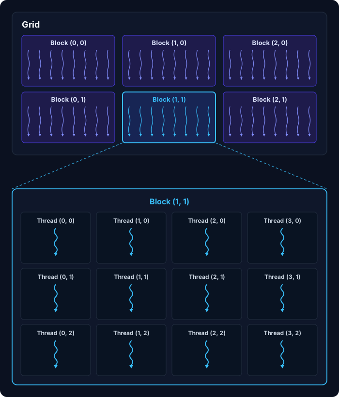CUDA Grid, Block, and Thread Hierarchy Figure 1: The CUDA programming model hierarchy. Kernels execute as a grid of thread blocks, which are partitioned by the hardware into 32-thread lockstep warps executed across physical Streaming Multiprocessors. Source: Wikimedia Commons (File:Block-thread.svg).

In SIMT:

The developer writes code for an individual thread executing scalar operations.
The compiler and GPU hardware automatically group 32 consecutive threads into a Warp.
A single instruction fetch and decode unit broadcasts one instruction to 32 parallel execution lanes simultaneously.
Each lane operates on private registers and distinct memory addresses, maintaining the illusion of independent scalar threads.

By sharing a single instruction fetch, decode, and dispatch pipeline across 32 threads, the GPU saves vast amounts of silicon die area that would otherwise be wasted on redundant control logic, dedicating that area directly to floating-point arithmetic.

2. Anatomy of the Hardware Warp Scheduler

Inside each SM sub-core sits a dedicated Hardware Warp Scheduler. Unlike an operating system thread scheduler on a CPU—which requires hundreds of cycles to save registers to stack memory and execute context switches—the GPU warp scheduler switches contexts with zero clock cycle overhead.

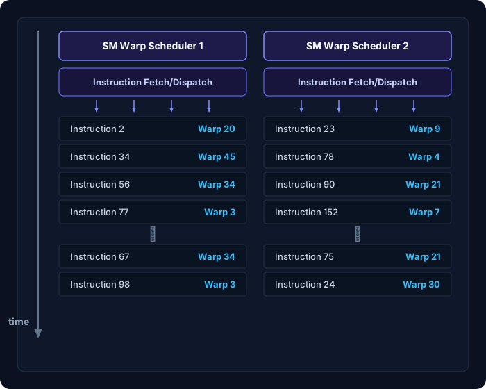Dual Warp Scheduler Architecture in NVIDIA GPUs Figure 2: Microarchitecture of a dual Warp Scheduler and Instruction Dispatch Unit. The scheduler monitors an active pool of warps and issues instructions to execution units every clock cycle without software intervention. Source: Wikimedia Commons (File:Warp-Scheduler-Gpu.jpg) / NVIDIA Fermi Whitepaper.

How Zero-Overhead Context Switching Works

Every warp resident on an SM has its architectural state permanently held in physical hardware:

Dedicated 32-bit registers allocated in the on-chip Register File.
A dedicated Program Counter (PC).
An active thread execution mask (a 32-bit bitmask indicating which lanes are active).

Because no register state needs to be saved or restored to main memory, context switching is purely an arbitration decision. At every clock cycle:

The scheduler scans its pool of resident warps (e.g., up to 16 warps per sub-core, 64 warps per SM).
It filters for warps whose instruction operands are ready (all memory dependencies resolved, execution pipelines free).
It selects one or two ready warps based on a scheduling policy and issues their next instruction into the datapath.

Common Scheduling Policies

Greedy-Then-Oldest (GTO): The scheduler prioritizes issuing instructions from the same warp as long as it remains ready. When that warp stalls on a memory fetch, the scheduler switches to the oldest stalled warp that just became ready. GTO maximizes cache locality in L1/Shared Memory.
Round-Robin (RR): The scheduler cycles evenly across all ready warps in sequence, distributing execution evenly.

flowchart TD
    classDef schedStyle fill:#1e1b4b,stroke:#818cf8,stroke-width:2px,color:#ffffff;
    classDef checkStyle fill:#0f172a,stroke:#38bdf8,stroke-width:2px,color:#ffffff;
    classDef issueStyle fill:#064e3b,stroke:#10b981,stroke-width:2px,color:#ffffff;

    subgraph Warp_Arbitration["Zero-Cycle Hardware Warp Arbitration Loop"]
        S1["Step 1: Inspect pool of resident warps on SM sub-core"]:::schedStyle
        S2["Step 2: Filter warps with ready operands & resolved memory dependencies"]:::checkStyle
        S3["Step 3: Apply GTO / Round-Robin arbitration priority"]:::checkStyle
        S4["Step 4: Issue 32-wide instruction to ALUs or Load/Store pipelines"]:::issueStyle
        S1 --> S2 --> S3 --> S4
    end

3. The Branch Divergence Trap

Because all 32 threads in a warp share a single Program Counter, they must execute the exact same instruction at the exact same physical clock cycle. But what happens when the developer introduces conditional logic?

__global__ void exampleKernel(float* data) {
    int tid = threadIdx.x;
    if (tid % 2 == 0) {
        data[tid] = data[tid] * 2.0f; // Path A (Even threads)
    } else {
        data[tid] = data[tid] + 5.0f; // Path B (Odd threads)
    }
}

In this code, threads 0, 2, 4… evaluate the conditional as true, while threads 1, 3, 5… evaluate it as false. Because there is only one instruction decoder for the warp, the hardware cannot execute both branches simultaneously.

Instead, the GPU triggers Branch Divergence Serialization:

flowchart TD
    classDef warpStyle fill:#0f172a,stroke:#38bdf8,stroke-width:2px,color:#ffffff;
    classDef activeStyle fill:#064e3b,stroke:#10b981,stroke-width:2px,color:#ffffff;
    classDef maskedStyle fill:#7f1d1d,stroke:#ef4444,stroke-width:2px,color:#ffffff;

    subgraph Divergence_Timeline["Hardware Serialization of Divergent Branch Paths"]
        D1["Cycle 1-10: Evaluate Condition -> Active Mask splits 50/50"]:::warpStyle
        D2["Cycle 11-30: Execute Path A -> Odd threads masked off (ALUs idle)"]:::activeStyle
        D3["Cycle 31-50: Execute Path B -> Even threads masked off (ALUs idle)"]:::maskedStyle
        D4["Cycle 51+: Reconvergence Point -> Mask restored to all 32 threads"]:::warpStyle
        D1 --> D2 --> D3 --> D4
    end

Path A Execution: The hardware sets the active execution mask to 0x55555555 (even lanes active). The multiplier ALUs execute data[tid] * 2.0f. The 16 odd lanes sit completely idle, consuming clock power without performing useful work.
Path B Execution: The hardware flips the active mask to 0xAAAAAAAA (odd lanes active). The adder ALUs execute data[tid] + 5.0f. The 16 even lanes now sit idle.
Reconvergence: At the end of the if-else block, the hardware reaches an automatic reconvergence barrier and restores the full 32-thread mask.

During this sequence, total arithmetic efficiency dropped to 50%. If an algorithm has 4 divergent branches nested inside a loop, execution efficiency can collapse to $12.5%$ or lower. Writing performant CUDA or Triton kernels requires structuring algorithms so that all 32 threads within a warp follow identical execution paths.

4. Register Files and Bank Conflicts

Modern GPUs provide massive register capacity—up to 256 KB of SRAM per SM. However, feeding 128 floating-point ALUs simultaneously with two or three 32-bit operands per cycle requires an enormous read bandwidth:

$$\text{Read Bandwidth} = 128 \text{ cores} \times 3 \text{ operands} \times 4 \text{ bytes} \times 2.0 \text{ GHz} \approx 3.07 \text{ TB/s per SM}$$

Across 144 SMs on a flagship Blackwell die, aggregate register read bandwidth exceeds 440 TB/s—vastly higher than any DRAM or cache interconnect on Earth.

To deliver this bandwidth without blowing up silicon die area, the register file is partitioned into multiple physical Banks (typically 4 or 8 banks).

flowchart TD
    classDef bankStyle fill:#1e1b4b,stroke:#818cf8,stroke-width:2px,color:#ffffff;
    classDef collStyle fill:#064e3b,stroke:#10b981,stroke-width:2px,color:#ffffff;

    subgraph Operand_Collection["Operand Collector Architecture"]
        B1["Instruction issued: R0 = R1 + R2 (Both registers in Bank 0)"]:::bankStyle
        B2["Bank Conflict detected: Bank 0 can only serve 1 read per cycle"]:::bankStyle
        B3["Cycle 1: Read R1 from Bank 0 -> Buffer in Operand Collector"]:::collStyle
        B4["Cycle 2: Read R2 from Bank 0 -> Instruction dispatched to ALU"]:::collStyle
        B1 --> B2 --> B3 --> B4
    end

When multiple source operands for an instruction reside within the same physical register bank, the hardware suffers a Register Bank Conflict. An internal structure called the Operand Collector must serialize the reads over multiple clock cycles before the instruction can be dispatched to the arithmetic pipeline. Modern compilers use sophisticated register allocation algorithms to distribute operands across different banks, avoiding serialization penalties.

5. Latency Hiding and Little’s Law

Why does a GPU need dozens of concurrent warps to achieve peak performance? The mathematical answer is given by Little’s Law, a foundational principle of queuing theory:

$$L = \lambda \times W$$

Adapted for computer architecture:

$$\text{Required Concurrency (Warps)} = \frac{\text{Memory Latency (Cycles)}}{\text{Throughput Interval (Cycles between instructions)}}$$

Consider an NVIDIA H100 executing a memory-bound kernel:

Global memory latency ($W$) across HBM3: approximately 300 clock cycles.
An SM sub-core can issue one instruction every cycle ($\text{Interval} = 1$).
To ensure that the arithmetic pipeline never sits idle waiting for memory loads, the hardware must maintain at least:

$$\text{Concurrency} = 300 \text{ cycles} \times 1 = 300 \text{ independent instructions in flight}$$

Since each warp instruction represents 32 parallel thread operations, the warp scheduler needs approximately 10 to 12 ready warps per sub-core (40 to 48 warps per SM) actively interleaved in the pipeline. When Warp 0 requests data from HBM, it sleeps for 300 cycles. Warps 1 through 11 execute their instructions in subsequent cycles. By the time Warp 11 finishes, Warp 0’s data has arrived, and it resumes execution with zero idle cycles on the ALU.

This explains why occupancy (the ratio of active warps to maximum possible warps) is a primary metric in GPU performance tuning. If a kernel uses too many registers or too much shared memory per block, occupancy drops, latency hiding fails, and the ALUs spend hundreds of cycles starving for data.

6. Architectural Simulation: Warp Scheduling & Divergence

The following Python script models and simulates an in-order hardware Warp Scheduler. It demonstrates how zero-overhead latency hiding keeps execution pipelines saturated during memory stalls, and measures the exact throughput penalty caused by branch divergence.

Click to expand runnable code script

"""
Warp Scheduler, Latency Hiding, and Branch Divergence Simulator.
Simulates clock-by-clock execution of warps across memory stalls and divergent branches.
"""

from dataclasses import dataclass
from typing import List, Optional

@dataclass
class Instruction:
    opcode: str
    latency_cycles: int
    is_memory: bool = False
    is_divergent: bool = False
    divergence_ratio: float = 1.0  # Fraction of active threads (e.g. 0.5 for 50% divergence)

@dataclass
class WarpState:
    warp_id: int
    pc: int = 0
    stalled_until_cycle: int = 0
    instructions: List[Instruction] = None

    @property
    def is_finished(self) -> bool:
        return self.pc >= len(self.instructions)

def simulate_warp_scheduler(warps: List[WarpState], max_cycles: int = 1000):
    current_cycle = 0
    total_useful_flops = 0
    total_wasted_alu_cycles = 0
    pipeline_idle_cycles = 0

    while current_cycle < max_cycles:
        # Check if all warps have finished
        if all(w.is_finished for w in warps):
            break

        # Greedy-Then-Oldest (GTO): Find first ready warp
        ready_warp: Optional[WarpState] = None
        for w in warps:
            if not w.is_finished and w.stalled_until_cycle <= current_cycle:
                ready_warp = w
                break

        if ready_warp is None:
            # Latency hiding failed: All warps stalled on memory/dependencies
            pipeline_idle_cycles += 1
            current_cycle += 1
            continue

        # Issue instruction from ready warp
        instr = ready_warp.instructions[ready_warp.pc]
        ready_warp.pc += 1

        if instr.is_divergent:
            # Divergent branch: Execution serialized across paths
            active_threads = int(32 * instr.divergence_ratio)
            idle_threads = 32 - active_threads
            total_useful_flops += active_threads
            total_wasted_alu_cycles += idle_threads
            # Divergent execution costs extra serialization cycles
            ready_warp.stalled_until_cycle = current_cycle + instr.latency_cycles * 2
        else:
            total_useful_flops += 32
            ready_warp.stalled_until_cycle = current_cycle + instr.latency_cycles

        current_cycle += 1

    total_possible_ops = current_cycle * 32
    efficiency = (total_useful_flops / total_possible_ops) * 100.0 if total_possible_ops > 0 else 0

    print("=" * 70)
    print("GPU Warp Execution & Latency Hiding Simulation")
    print("=" * 70)
    print(f"Total Clock Cycles:          {current_cycle}")
    print(f"Pipeline Idle Cycles (Starve): {pipeline_idle_cycles} ({pipeline_idle_cycles/current_cycle*100:.1f}%)")
    print(f"Useful Thread Operations:    {total_useful_flops}")
    print(f"Wasted Operations (Masked):  {total_wasted_alu_cycles}")
    print(f"Overall Hardware Efficiency: {efficiency:.2f}%")
    print("=" * 70 + "\n")

def main():
    # Scenario A: Ideal parallel execution with latency hiding (16 warps interleaving memory loads)
    kernel_ideal = [
        Instruction("GLOBAL_LOAD", latency_cycles=20, is_memory=True),
        Instruction("FFMA", latency_cycles=4),
        Instruction("FFMA", latency_cycles=4),
        Instruction("GLOBAL_STORE", latency_cycles=10, is_memory=True)
    ]
    warps_a = [WarpState(warp_id=i, instructions=list(kernel_ideal)) for i in range(12)]
    print("SCENARIO A: Well-Interleaved Warps (Effective Latency Hiding)")
    simulate_warp_scheduler(warps_a)

    # Scenario B: High Branch Divergence (50% threads masked on branches)
    kernel_divergent = [
        Instruction("BRANCH_DIV", latency_cycles=4, is_divergent=True, divergence_ratio=0.5),
        Instruction("BRANCH_DIV", latency_cycles=4, is_divergent=True, divergence_ratio=0.25),
        Instruction("FFMA", latency_cycles=4),
        Instruction("GLOBAL_STORE", latency_cycles=10, is_memory=True)
    ]
    warps_b = [WarpState(warp_id=i, instructions=list(kernel_divergent)) for i in range(4)]
    print("SCENARIO B: Severe Branch Divergence & Low Occupancy")
    simulate_warp_scheduler(warps_b)

if __name__ == "__main__":
    main()

What’s Next in the Series?

Now that we have understood how Streaming Multiprocessors orchestrate warps and registers within a single monolithic chip, we are ready to explore the greatest manufacturing transformation in modern computing history.

In Part 7: Advanced Packaging & The Chiplet Era: CoWoS, 3D Stacking, and Interposers, we will investigate what happens when modern AI models become too large to fit on a single reticle-limited silicon die: TSMC CoWoS, silicon interposers, High Bandwidth Memory (HBM) stacking, and NVIDIA’s 10 TB/s NV-HBI chiplet bridge.