
The 3D Gaussian Splatting Revolution: Real-Time Differentiable Primitives
Explore the 3D Gaussian Splatting revolution: explicit covariance parameterization, Spherical Harmonics, GPU tile rasterization, and 100+ FPS rendering.
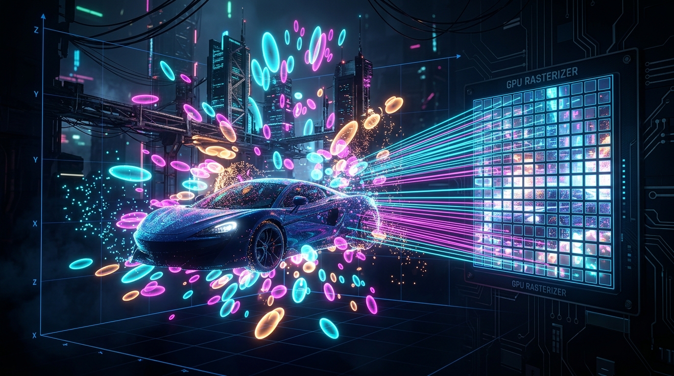
Series: NVIDIA Physical AI & Robotics Ecosystem Series - Part 14
Series: ← Part 13: Accelerating Implicit Fields: Instant-NGP & Multiresolution Hash Grids (Previous) Series: Part 15: NVIDIA NuRec & Dynamic 3DGS: Photorealistic Digital Twins for Robotics & AV Simulation (Next) →
Prior Reading Material
Before diving into differentiable rasterization and anisotropic Gaussian primitives, review these foundational articles across our Physical AI and Computer Vision series:
- Part 1: Unpacking the NVIDIA Physical AI Data Factory (PAIDF) Stack — Synthetic data generation and spatial computing pipelines.
- Part 3: Unlocking NVIDIA Omniverse: Architecture, OpenUSD, RTX Rendering, and the Industrial Metaverse Ecosystem — GPU path tracing and real-time volumetric scene composition.
- Part 5: Scaling Physics with Isaac Sim & Omniverse Replicator — Ray-traced sensor synthesis and GPU-accelerated domain randomization.
- Part 12: Demystifying NeRFs: Volumetric Rendering & Implicit Coordinate Networks — Continuous 5D coordinate networks, Fourier positional encodings, and numerical volumetric quadrature.
- Part 13: Accelerating Implicit Fields: Instant-NGP & Multiresolution Hash Grids — Multiresolution spatial hash tables, occupancy bitmasks, and tiny fully-fused CUDA MLPs.
Official Research & Project Summary
| Dimension / Component | Specifications & Research Details |
|---|---|
| Foundational Research Paper | 3D Gaussian Splatting for Real-Time Radiance Field Rendering (Kerbl et al., SIGGRAPH 2023) |
| Primary Open-Source Repositories | graphdeco-inria/gaussian-splatting, nerfstudio-project/gsplat |
| Interactive Viewers & Runtimes | SIBR_viewers (Inria), PlayCanvas WebGL Gaussian Viewer |
| Geometric Primitive Type | Explicit Parameterized Anisotropic 3D Gaussians $(\boldsymbol{\mu}, \boldsymbol{\Sigma}, \alpha, \mathbf{c}_{SH})$ |
| Rendering Primitive | Tile-Based Differentiable GPU Radix Sort & Alpha-Blending Rasterization |
| Inference Throughput (1080p / 4K) | ⚡ 100–250+ FPS (Sub-5ms per 4K frame on modern RTX GPUs) |
| Training Duration (COLMAP Initialization) | ⚡ 15–30 Minutes (30,000 optimization iterations) |
1. The Paradigm Shift: From Volumetric Fog to Glowing Ellipsoids
For three years following the release of NeRF in 2020, neural rendering was dominated by implicit continuous representations: shooting virtual camera rays into space and integrating numerical optical densities through neural networks.
Even with the multi-thousand-fold acceleration of Instant-NGP, the fundamental bottleneck remained: ray marching. Every pixel required stepping through 3D space, computing trilinear interpolation weights, and accumulating transmittance.
flowchart TD
    A["The Neural Rendering Paradigm Shift"] --> B["The Implicit Fog Paradigm (NeRF / Instant-NGP)"]
    A --> C["The Explicit Primitive Paradigm (3D Gaussian Splatting)"]

    B --> B1["Shoot Camera Rays through Every Pixel Frustum"]
    B --> B2["Sample Hundreds of Points per Ray along Camera Axis"]
    B --> B3["Evaluate Neural Weights or Hash Tables at Every Step"]
    B --> B4["Rendering Bound by Ray Traversal Complexity (~15-30 FPS)"]

    C --> C1["Populate Scene with Millions of Explicit 3D Glowing Ellipsoids"]
    C --> C2["Project 3D Ellipsoids directly onto 2D Screen Sensor (EWA Splatting)"]
    C --> C3["Assign Gaussians to 16x16 GPU Screen Tiles & Radix Sort by Depth"]
    C --> C4["Unleash Native GPU Hardware Rasterization (100-250+ FPS)"]

    style A fill:#0d2b45,stroke:#00e5ff,stroke-width:2px,color:#ffffff
    style B fill:#1e293b,stroke:#94a3b8,stroke-width:1px,color:#ffffff
    style C fill:#064e3b,stroke:#34d399,stroke-width:2px,color:#ffffff
    style B1 fill:#0f172a,stroke:#38bdf8,stroke-width:1px,color:#ffffff
    style B2 fill:#0f172a,stroke:#38bdf8,stroke-width:1px,color:#ffffff
    style B3 fill:#0f172a,stroke:#38bdf8,stroke-width:1px,color:#ffffff
    style B4 fill:#3b0764,stroke:#e879f9,stroke-width:2px,color:#ffffff
    style C1 fill:#0f172a,stroke:#38bdf8,stroke-width:1px,color:#ffffff
    style C2 fill:#0f172a,stroke:#38bdf8,stroke-width:1px,color:#ffffff
    style C3 fill:#0f172a,stroke:#38bdf8,stroke-width:1px,color:#ffffff
    style C4 fill:#064e3b,stroke:#34d399,stroke-width:2px,color:#ffffff
In 2023, Bernhard Kerbl, Georgios Kopanas, Thomas Leimkühler, and George Drettakis published 3D Gaussian Splatting (3DGS).
3DGS inverted the rendering equation:
- Instead of casting rays into an invisible volume, 3DGS models the scene as millions of explicit, translucent 3D ellipsoidal Gaussian paint droplets.
- Modern GPUs project these ellipsoids directly onto the 2D camera plane and composite them in parallel using lightning-fast tile-based GPU radix sorting.
- The result is the exact visual photorealism of continuous NeRFs, rendered in real time at over 100 frames per second at 4K resolution.
2. The Anatomy of a 3D Gaussian Primitive
Every object in a 3DGS scene is composed of an ensemble of anisotropic (non-spherical) 3D Gaussians. Each individual Gaussian $i$ is parameterized by four distinct geometric and radiometric attributes:
flowchart TD
    G["Parametric 3D Gaussian Primitive (Gaussian i)"] --> G1["1. Center Position: mu = (x, y, z) in R^3"]
    G --> G2["2. 3D Covariance Matrix: Sigma in R^(3x3) (Orientation & Scale)"]
    G --> G3["3. Base Opacity: alpha in [0, 1] (Differential Transparency)"]
    G --> G4["4. Spherical Harmonics: c_SH in R^(16x3) (View-Dependent Radiance)"]

    G2 --> G2A["Scale Vector: s = (s_x, s_y, s_z) in Log-Space"]
    G2 --> G2B["Unit Quaternion Rotation: q = (w, x, y, z) in S^3"]
    G2A --> G2C["Factorization: Sigma = R S S^T R^T (Guarantees Positive Semi-Definiteness)"]
    G2B --> G2C

    style G fill:#0d2b45,stroke:#00e5ff,stroke-width:2px,color:#ffffff
    style G1 fill:#0f172a,stroke:#38bdf8,stroke-width:1px,color:#ffffff
    style G2 fill:#0f172a,stroke:#38bdf8,stroke-width:1px,color:#ffffff
    style G3 fill:#0f172a,stroke:#38bdf8,stroke-width:1px,color:#ffffff
    style G4 fill:#0f172a,stroke:#38bdf8,stroke-width:1px,color:#ffffff
    style G2A fill:#1e293b,stroke:#94a3b8,stroke-width:1px,color:#ffffff
    style G2B fill:#1e293b,stroke:#94a3b8,stroke-width:1px,color:#ffffff
    style G2C fill:#064e3b,stroke:#34d399,stroke-width:2px,color:#ffffff
1. Spatial Probability Density Function
A 3D Gaussian centered at mean position $\boldsymbol{\mu} \in \mathbb{R}^3$ evaluates the continuous spatial density:
$$ G(\mathbf{x}) = \exp\left( -\frac{1}{2} (\mathbf{x} - \boldsymbol{\mu})^T \boldsymbol{\Sigma}^{-1} (\mathbf{x} - \boldsymbol{\mu}) \right) $$
Where $\boldsymbol{\Sigma} \in \mathbb{R}^{3 \times 3}$ is the 3D covariance matrix describing the ellipsoid’s three-dimensional dimensions and spatial tilt.
2. Covariance Factorization: $\boldsymbol{\Sigma} = \mathbf{R} \mathbf{S} \mathbf{S}^T \mathbf{R}^T$
During gradient descent, optimizing a $3 \times 3$ covariance matrix directly is dangerous: covariance matrices must remain positive semi-definite (PSD) at all times ($\det(\boldsymbol{\Sigma}) > 0$). If optimization produces a non-PSD matrix, the Gaussian collapses or produces imaginary spatial radii.
To guarantee physical validity throughout optimization without complex constrained optimization, 3DGS factorizes $\boldsymbol{\Sigma}$ into scaling $\mathbf{S}$ and rotation $\mathbf{R}$:
$$ \boldsymbol{\Sigma} = \mathbf{R} \mathbf{S} \mathbf{S}^T \mathbf{R}^T $$
Where:
- $\mathbf{S} = \operatorname{diag}(s_x, s_y, s_z)$ is stored as 3 unconstrained real numbers in log-space ($s_i = \exp(\ell_i)$), guaranteeing strictly positive scale axes.
- $\mathbf{R}$ is parameterized by a normalized 4D unit quaternion $\mathbf{q} = (w, x, y, z)$, which is converted into an orthogonal $3 \times 3$ rotation matrix during the forward pass.
3. View-Dependent Radiance with Spherical Harmonics (SH)
Just as NeRF conditions color on the camera viewing angle, 3D Gaussians capture glossy specular highlights, anisotropic reflections, and Fresnel sheen using Spherical Harmonics (SH) basis functions:
$$ \mathbf{c}(\mathbf{d}) = \sum_{\ell=0}^{L_{\max}} \sum_{m=-\ell}^{\ell} c_\ell^m Y_\ell^m(\mathbf{d}) $$
Where $Y_\ell^m(\mathbf{d})$ are the real spherical harmonic basis functions evaluated on viewing direction unit vector $\mathbf{d} \in \mathbb{S}^2$.
By setting maximum degree $L_{\max} = 3$, each Gaussian stores $(3+1)^2 = 16$ coefficient vectors (48 floating-point numbers for RGB). Degree $0$ captures diffuse base color, while degrees $1, 2, 3$ synthesize metallic sheens that change dynamically as the camera moves.
3. Tile-Based Differentiable GPU Rasterization
The defining breakthrough of 3DGS is its tile-based differentiable GPU rasterizer, which bypasses ray marching entirely by leveraging modern GPU graphics hardware architectures.
flowchart TD
    R1["Initialize Camera View Matrix W and Projection Matrix P"] --> R2["Frustum Culling: Discard Gaussians Outside Camera Frustum"]
    R2 --> R3["2D Screen Projection (EWA Splatting): Compute Screen Covariance Sigma'"]
    R3 --> R4["Screen Space Tiling: Divide 1920x1080 Screen into 16x16 Pixel Tiles"]
    R4 --> R5["Instantiate 64-bit Key-Value Pairs per Gaussian: Tile ID (32-bit) | Depth z (32-bit)"]
    R5 --> R6["GPU Radix Sort (CUB): Sort Millions of Gaussians Front-to-Back Globally in Sub-ms"]
    R6 --> R7["Per-Tile Threadblock Execution: Load Sorted Gaussians into Fast Shared Memory"]
    R7 --> R8["Front-to-Back Alpha Compositing with Early Transmittance Termination (T < 1e-4)"]
    R8 --> R9["Render Final 100+ FPS Photorealistic 4K Image"]

    style R1 fill:#0d2b45,stroke:#00e5ff,stroke-width:2px,color:#ffffff
    style R2 fill:#0f172a,stroke:#38bdf8,stroke-width:1px,color:#ffffff
    style R3 fill:#0f172a,stroke:#38bdf8,stroke-width:1px,color:#ffffff
    style R4 fill:#0f172a,stroke:#38bdf8,stroke-width:1px,color:#ffffff
    style R5 fill:#1e293b,stroke:#94a3b8,stroke-width:1px,color:#ffffff
    style R6 fill:#3b0764,stroke:#e879f9,stroke-width:2px,color:#ffffff
    style R7 fill:#0f172a,stroke:#38bdf8,stroke-width:1px,color:#ffffff
    style R8 fill:#064e3b,stroke:#34d399,stroke-width:2px,color:#ffffff
    style R9 fill:#064e3b,stroke:#34d399,stroke-width:2px,color:#ffffff
The 2D Projection: EWA Splatting
To project a 3D Gaussian onto the camera sensor plane, 3DGS applies Elliptical Weighted Average (EWA) splatting (Zwicker et al., 2001).
Given camera extrinsic viewing matrix $\mathbf{W}$ and projective transformation Jacobian $\mathbf{J}$, the 2D projected screen covariance $\boldsymbol{\Sigma}’ \in \mathbb{R}^{2 \times 2}$ is:
$$ \boldsymbol{\Sigma}’ = \mathbf{J} \mathbf{W} \boldsymbol{\Sigma} \mathbf{W}^T \mathbf{J}^T $$
To prevent aliasing when a Gaussian projects smaller than a single pixel, a low-pass filtering term $+0.3 \mathbf{I}_{2 \times 2}$ is added to the diagonal of $\boldsymbol{\Sigma}’$.
GPU Radix Sorting in One Pass
- The screen is divided into uniform $16 \times 16$ pixel tiles.
- For each Gaussian overlapping a tile, a 64-bit sorting key is created: $$\text{Key} = \left[ \text{Tile ID (Bits 32–63)} ; \vert ; \text{View-Space Depth } z \text{ (Bits 0–31)} \right]$$
- A single call to NVIDIA’s high-speed GPU Radix Sort (
cub::DeviceRadixSort) sorts millions of Gaussians across all tiles simultaneously in under 0.5 milliseconds. - Each $16 \times 16$ tile launches a CUDA threadblock. Pixels in the tile load the pre-sorted Gaussians into fast on-chip shared memory (SRAM) and evaluate front-to-back alpha compositing in parallel.
4. Adaptive Density Control: Splitting, Cloning, and Pruning
Starting from a sparse point cloud generated by Structure-from-Motion (COLMAP), 3DGS must autonomously populate empty regions and refine complex geometry.
Every $100$ optimization steps, 3DGS inspects the average positional gradient norm $|\nabla_{\boldsymbol{\mu}} \mathcal{L}|_2$ for every Gaussian:
flowchart TD
    A1["Every 100 Steps: Check Positional Gradient Magnitude"] --> A2{"Is Average Gradient > Threshold tau_pos?"}
    A2 -- No --> A3["Maintain Gaussian Unchanged"]
    A2 -- Yes --> A4{"Is Gaussian Scale s > Spatial Threshold tau_scale?"}

    A4 -- Yes: Over-Reconstruction --> A5["SPLIT: Replace 1 Large Gaussian with 2 Smaller Gaussians (Scale / 1.6)"]
    A4 -- No: Under-Reconstruction --> A6["CLONE: Duplicate Gaussian and Shift along Gradient Direction"]

    A5 --> A7["Pruning Pass: Delete Gaussians with Opacity alpha < 0.005 or Oversized Radii"]
    A6 --> A7
    A3 --> A7

    A7 --> A8["Every 3,000 Iterations: Reset Opacity alpha to Near-Zero (Eliminates Transparent Floaters)"]

    style A1 fill:#0d2b45,stroke:#00e5ff,stroke-width:2px,color:#ffffff
    style A2 fill:#0f172a,stroke:#38bdf8,stroke-width:1px,color:#ffffff
    style A3 fill:#1e293b,stroke:#94a3b8,stroke-width:1px,color:#ffffff
    style A4 fill:#0f172a,stroke:#38bdf8,stroke-width:1px,color:#ffffff
    style A5 fill:#3b0764,stroke:#e879f9,stroke-width:2px,color:#ffffff
    style A6 fill:#3b0764,stroke:#e879f9,stroke-width:2px,color:#ffffff
    style A7 fill:#0f172a,stroke:#38bdf8,stroke-width:1px,color:#ffffff
style A8 fill:#064e3b,stroke:#34d399,stroke-width:2px,color:#ffffff- Under-Reconstruction (Cloning): If an object region lacks geometric primitives (small scale $s < \tau_s$ but high gradient), the Gaussian is cloned and shifted along the gradient vector to fill the geometric void.
- Over-Reconstruction (Splitting): If a single large Gaussian covers an intricate geometric surface (large scale $s > \tau_s$ and high gradient), it is split into two smaller Gaussians whose scale is divided by $1.6$, dividing the representation into finer details.
- Opacity Resetting & Pruning: Gaussians with opacity $\alpha < 0.005$ are pruned. Every $3{,}000$ steps, all opacities are reset to near-zero ($\alpha = 0.01$), forcing the optimizer to re-justify their existence and ruthlessly destroying transparent “floaters”.
5. Formal Mathematical Formulations
Alpha-Compositing of Projected 2D Gaussians
For a pixel coordinate $p \in \mathbb{R}^2$, let $\mathcal{N}$ denote the ordered set of $M$ overlapping Gaussians sorted front-to-back by camera depth ($z_1 \le z_2 \le \dots \le z_M$). The rendered pixel color $C(p)$ is computed as:
$$ C(p) = \sum_{i \in \mathcal{N}} \mathbf{c}i \alpha_i(p) \prod{j=1}^{i-1} \left( 1 - \alpha_j(p) \right) $$
Where the pixel-specific opacity $\alpha_i(p)$ evaluates the 2D projected Gaussian profile multiplied by learned base opacity $o_i \in [0, 1]$:
$$ \alpha_i(p) = o_i \exp\left( -\frac{1}{2} (p - \boldsymbol{\mu}‘_i)^T (\boldsymbol{\Sigma}‘_i)^{-1} (p - \boldsymbol{\mu}‘_i) \right) $$
Where $\boldsymbol{\mu}‘_i \in \mathbb{R}^2$ is the projected 2D screen center, and $\boldsymbol{\Sigma}‘_i \in \mathbb{R}^{2 \times 2}$ is the 2D screen covariance.
Composite Training Loss Function
3DGS is optimized end-to-end by minimizing a combined $\mathcal{L}_1$ pixel error and Structural Similarity (D-SSIM) metric:
$$ \mathcal{L} = (1 - \lambda) \mathcal{L}1(\hat{C}, C{gt}) + \lambda \mathcal{L}{\text{D-SSIM}}(\hat{C}, C{gt}) $$
Where:
- $\mathcal{L}1(\hat{C}, C{gt}) = \frac{1}{|P|} \sum_{p \in P} |\hat{C}(p) - C_{gt}(p)|$
- $\mathcal{L}{\text{D-SSIM}}(\hat{C}, C{gt}) = 1 - \operatorname{SSIM}(\hat{C}, C_{gt})$
- Standard weighting parameter $\lambda = 0.2$.
6. Interactive Python Simulation: 3DGS Projection, Radix Sorting & Alpha-Blending
To inspect quaternion covariance factorization, 2D screen projection, and depth-sorted tile rasterization, run the zero-dependency Python script below.
Click to expand runnable Python simulation script
#!/usr/bin/env python3
"""
3D Gaussian Splatting Simulation: Covariance Factorization, EWA Screen Projection, & Tile Rasterization.
Zero external dependencies (pure Python standard library).
"""

import math
import random

class Gaussian3D:
    """Represents an anisotropic 3D Gaussian primitive."""
    def __init__(self, gid: str, mean: tuple, scales: tuple, quaternion: tuple, opacity: float, color: tuple):
        self.gid = gid
        self.mean = mean # (x, y, z)
        self.scales = scales # (sx, sy, sz)
        self.q = quaternion # (w, x, y, z)
        self.opacity = opacity
        self.color = color # (r, g, b)

    def compute_rotation_matrix(self) -> list:
        """Converts normalized unit quaternion (w, x, y, z) to 3x3 rotation matrix R."""
        w, x, y, z = self.q
        norm = math.sqrt(w*w + x*x + y*y + z*z)
        w, x, y, z = w/norm, x/norm, y/norm, z/norm

        return [
            [1 - 2*(y*y + z*z), 2*(x*y - w*z),     2*(x*z + w*y)],
            [2*(x*y + w*z),     1 - 2*(x*x + z*z), 2*(y*z - w*x)],
            [2*(x*z - w*y),     2*(y*z + w*x),     1 - 2*(x*x + y*y)]
        ]

    def compute_3d_covariance(self) -> list:
        """Factorizes Sigma = R * S * S^T * R^T to guarantee positive semi-definiteness."""
        R = self.compute_rotation_matrix()
        sx, sy, sz = self.scales

        # M = R * S
        M = [
            [R[0][0]*sx, R[0][1]*sy, R[0][2]*sz],
            [R[1][0]*sx, R[1][1]*sy, R[1][2]*sz],
            [R[2][0]*sx, R[2][1]*sy, R[2][2]*sz]
        ]

        # Sigma = M * M^T
        Sigma = [[0.0]*3 for _ in range(3)]
        for i in range(3):
            for j in range(3):
                Sigma[i][j] = round(sum(M[i][k] * M[j][k] for k in range(3)), 4)
        return Sigma

    def project_to_screen_ewa(self, focal_length: float = 500.0) -> dict:
        """Projects 3D Gaussian to 2D screen covariance Sigma' using EWA Splatting."""
        x, y, z = self.mean
        if z <= 0.1:
            return None # Behind camera

        # 2D Screen Center
        px = focal_length * (x / z) + 400.0 # 800x800 resolution center
        py = focal_length * (y / z) + 400.0

        # Approximate 2D covariance diagonal from scale and depth
        Sigma_3d = self.compute_3d_covariance()
        inv_z = 1.0 / z
        inv_z2 = inv_z * inv_z

        # Projected 2D covariance + 0.3 low-pass pixel filter
        sigma_xx = round(focal_length**2 * inv_z2 * (Sigma_3d[0][0] + (x/z)**2 * Sigma_3d[2][2]) + 0.3, 3)
        sigma_yy = round(focal_length**2 * inv_z2 * (Sigma_3d[1][1] + (y/z)**2 * Sigma_3d[2][2]) + 0.3, 3)
        sigma_xy = round(focal_length**2 * inv_z2 * (Sigma_3d[0][1]), 3)

        return {
            "gid": self.gid,
            "screen_pos": (round(px, 2), round(py, 2)),
            "depth_z": round(z, 3),
            "cov_2d": [[sigma_xx, sigma_xy], [sigma_xy, sigma_yy]],
            "opacity": self.opacity,
            "color": self.color
        }


class TileRasterizer:
    """Simulates 16x16 GPU tile binning, depth sorting, and alpha-blending."""
    def __init__(self, tile_size: int = 16):
        self.tile_size = tile_size

    def render_pixel(self, projected_gaussians: list, target_pixel: tuple) -> dict:
        px, py = target_pixel
        overlapping = []

        for g in projected_gaussians:
            gx, gy = g["screen_pos"]
            dx = px - gx
            dy = py - gy
            cov = g["cov_2d"]

            # Determinant of 2x2 covariance
            det = cov[0][0]*cov[1][1] - cov[0][1]*cov[1][0]
            if det <= 1e-4:
                continue

            # Inverse covariance
            inv_cov = [
                [cov[1][1] / det, -cov[0][1] / det],
                [-cov[1][0] / det, cov[0][0] / det]
            ]

            # Mahalanobis power: 0.5 * d^T * inv_cov * d
            power = 0.5 * (dx * (inv_cov[0][0]*dx + inv_cov[0][1]*dy) + dy * (inv_cov[1][0]*dx + inv_cov[1][1]*dy))

            if power <= 4.5: # Inside 3-sigma bounding ellipse
                gaussian_profile = math.exp(-power)
                alpha_sample = g["opacity"] * gaussian_profile
                overlapping.append({
                    "gid": g["gid"],
                    "depth_z": g["depth_z"],
                    "alpha": round(alpha_sample, 4),
                    "color": g["color"]
                })

        # GPU Radix Sort: Sort ascending by depth (front-to-back)
        overlapping.sort(key=lambda item: item["depth_z"])

        # Alpha compositing
        accumulated_rgb = [0.0, 0.0, 0.0]
        transmittance = 1.0
        blend_logs = []

        for item in overlapping:
            alpha = item["alpha"]
            weight = transmittance * alpha
            r, g, b = item["color"]

            accumulated_rgb[0] += weight * r
            accumulated_rgb[1] += weight * g
            accumulated_rgb[2] += weight * b

            blend_logs.append({
                "gid": item["gid"],
                "z": item["depth_z"],
                "alpha": alpha,
                "weight": round(weight, 4),
                "transmittance_left": round(transmittance * (1.0 - alpha), 4)
            })

            transmittance *= (1.0 - alpha)
            if transmittance < 1e-4:
                break

        return {
            "pixel": target_pixel,
            "rendered_rgb": [round(c, 4) for c in accumulated_rgb],
            "final_transmittance": round(transmittance, 4),
            "blending_steps": blend_logs
        }


def main():
    print("=" * 80)
    print("1. 3D GAUSSIAN SPLATTING: COVARIANCE FACTORIZATION & 2D PROJECTION")
    print("=" * 80)

    # 3 Synthetic Gaussians
    g1 = Gaussian3D("G_Amber", mean=(0.1, 0.1, 2.5), scales=(0.2, 0.08, 0.1), quaternion=(1.0, 0.2, 0.0, 0.1), opacity=0.9, color=(1.0, 0.6, 0.1))
    g2 = Gaussian3D("G_Cyan",  mean=(0.12, 0.08, 3.2), scales=(0.3, 0.15, 0.1), quaternion=(0.9, 0.0, 0.3, 0.0), opacity=0.85, color=(0.0, 0.9, 1.0))
    g3 = Gaussian3D("G_Magenta", mean=(0.08, 0.14, 1.8), scales=(0.15, 0.15, 0.15), quaternion=(1.0, 0.0, 0.0, 0.0), opacity=0.95, color=(1.0, 0.2, 0.8))

    gaussians = [g1, g2, g3]
    projected = [g.project_to_screen_ewa() for g in gaussians if g.project_to_screen_ewa() is not None]

    print(f"{'Gaussian ID':<12}{'World (x,y,z)':<20}{'Screen Center (px,py)':<24}{'Depth z':<10}{'2D Covariance'}")
    print("-" * 80)
    for g, p in zip(gaussians, projected):
        print(f"{g.gid:<12}{str(g.mean):<20}{str(p['screen_pos']):<24}{p['depth_z']:<10}{p['cov_2d']}")
    print("-" * 80)

    print("\n" + "=" * 80)
    print("2. GPU TILE RADIX SORT & PARALLEL ALPHA-COMPOSITING SIMULATION")
    print("=" * 80)

    target_pixel = (420.0, 420.0)
    rasterizer = TileRasterizer()
    res = rasterizer.render_pixel(projected, target_pixel)

    print(f"Target Screen Pixel Coordinate: {target_pixel}")
    print(f"{'Rank / ID':<14}{'Depth (z)':<12}{'Sample Alpha':<14}{'Blending Weight':<18}{'Transmittance Remaining'}")
    print("-" * 80)
    for step in res["blending_steps"]:
        print(f"{step['gid']:<14}{step['z']:<12}{step['alpha']:<14}{step['weight']:<18}{step['transmittance_left']}")
    print("-" * 80)
    print(f"Synthesized 3DGS Pixel Color RGB : {res['rendered_rgb']}")
    print(f"Unoccluded Background Visibility : {res['final_transmittance']}")
    print("=" * 80)

if __name__ == "__main__":
    main()
7. Summary & The Road to Robotics Digital Twins
3D Gaussian Splatting transformed computer graphics by proving that neural view synthesis could achieve real-time rendering:
- Explicit Differentiable Primitives: Replacing continuous MLPs with parameterized 3D ellipsoids factorized via $\boldsymbol{\Sigma} = \mathbf{R}\mathbf{S}\mathbf{S}^T\mathbf{R}^T$ eliminates gradient collapse.
- Tile-Based GPU Radix Sorting: Binning Gaussians into $16 \times 16$ pixel tiles enables 100+ FPS photorealistic rendering on modern GPUs.
- Adaptive Density Optimization: Dynamically cloning under-reconstructed geometry, splitting over-reconstructed primitives, and pruning floaters generates sharp, photorealistic 3D worlds.
The Next Frontier: Dynamic Physical AI Digital Twins
While static 3DGS accurately reconstructs stationary scenes, physical AI and autonomous vehicles require modeling dynamic worlds with moving vehicles, walking pedestrians, and deformable objects.
In Part 15, we explore NVIDIA NuRec (Neural Reconstruction), showing how NVIDIA integrates dynamic 3DGS with multi-camera, LiDAR, and IMU drive logs inside NVIDIA Omniverse & DRIVE Sim to create reactive closed-loop simulation environments.
Series Navigation
Series: ← Part 13: Accelerating Implicit Fields: Instant-NGP & Multiresolution Hash Grids (Previous) Series: Part 15: NVIDIA NuRec & Dynamic 3DGS: Photorealistic Digital Twins for Robotics & AV Simulation (Next) →