
Demystifying NeRFs: Volumetric Rendering & Implicit Coordinate Networks
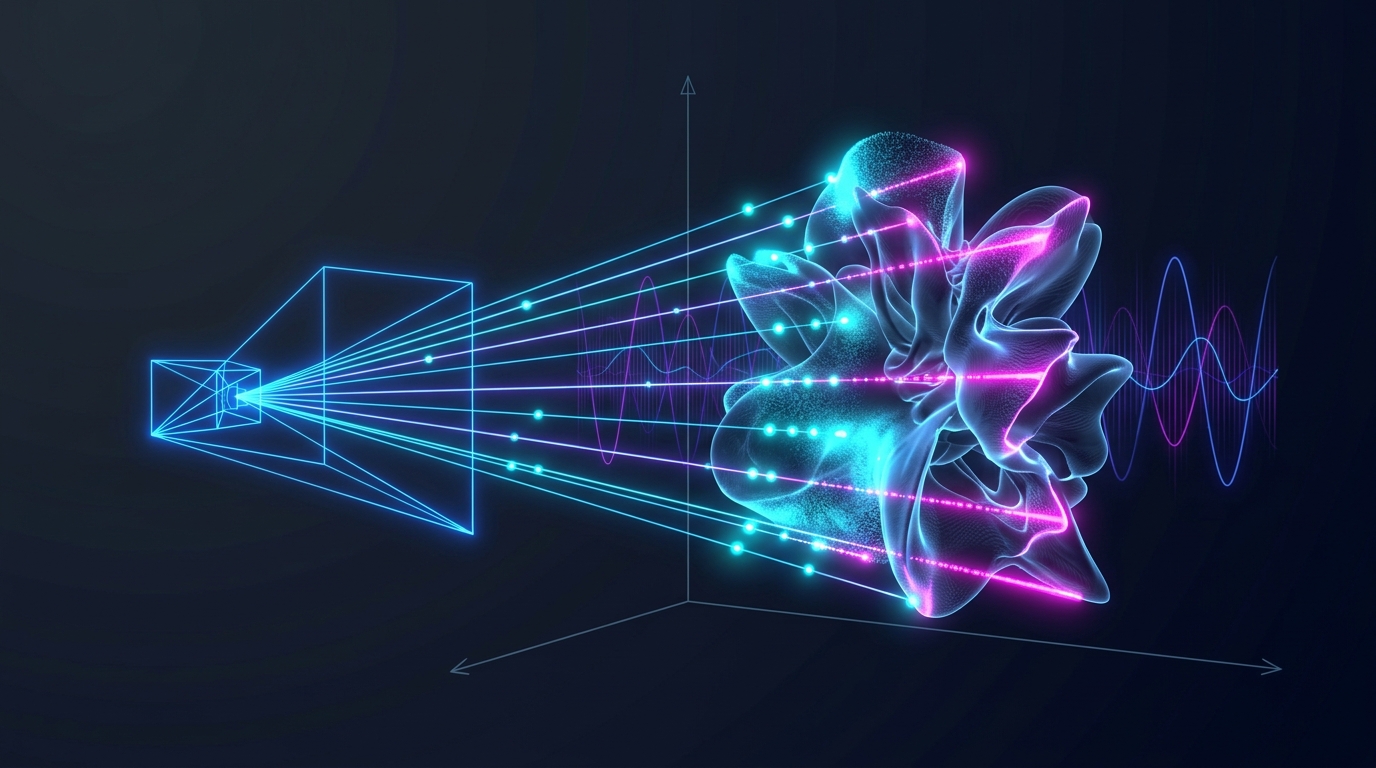
Explore the mechanics of Neural Radiance Fields (NeRFs), from 5D continuous coordinate networks and positional encodings to numerical volumetric quadrature.
Series: NVIDIA Physical AI & Robotics Ecosystem Series - Part 12
Series: ← Part 11: NVIDIA Drive Cosmos & Cosmos-Drive-Dreams: Scalable Synthetic Driving Data Generation with World Foundation Models (Previous) Series: Part 13: Accelerating Implicit Fields: Instant-NGP & Multiresolution Hash Grids (Next) →
Prior Reading Material
Before exploring implicit neural representations and volumetric ray marching, inspect these foundational articles from our Physical AI and Computer Vision series:
- Part 1: Unpacking the NVIDIA Physical AI Data Factory (PAIDF) Stack — The complete end-to-end synthetic data and physical intelligence pipeline.
- Part 2: Inside NVIDIA Cosmos: World Foundation Models for Physical Commonsense — Physics-conditioned video generation and 3D spatiotemporal tokenizers.
- Part 3: Unlocking NVIDIA Omniverse: Architecture, OpenUSD, RTX Rendering, and the Industrial Metaverse Ecosystem — Real-time ray tracing, path tracing, and universal 3D scene representation.
- Part 4: Demystifying OpenUSD: Architecture, Composition Arcs, usdview, and Simulation Assets — Core geometric and asset composition principles in spatial workflows.
- Part 5: Scaling Physics with Isaac Sim & Omniverse Replicator — Ray-traced sensor synthesis (LiDAR, RGB, depth) and automated domain randomization.
- Part 9: The Evolutionary Arc of Computer Vision: From LeNet-5 and ResNet to ConvNeXt and 3D Video Models — From 2D spatial convolutions to spatiotemporal 3D vision.
- Part 11: NVIDIA Drive Cosmos & Cosmos-Drive-Dreams: Scalable Synthetic Driving Data Generation with World Foundation Models — Scalable multi-view synthetic sensor generation for autonomous physical agents.
Official Research & Project Summary
| Milestone / Paradigm | Key Research Papers | Primary Open-Source Implementations | Representation Type | 1080p Novel View Synthesis Speed |
|---|---|---|---|---|
| Vanilla NeRF | Mildenhall et al., ECCV 2020 | nerf-pytorch, nerfstudio | Implicit Continuous MLP: $F_\Theta(\mathbf{x}, \mathbf{d}) \to (\mathbf{c}, \sigma)$ | ❌ Very Slow (~0.1 FPS) |
| Mip-NeRF | Barron et al., ICCV 2021 | google-research/multinerf | Anti-Aliased Cone Frustum Tracing MLP | ❌ Very Slow (~0.08 FPS) |
| RawNeRF | Mildenhall et al., CVPR 2022 | google-research/multinerf | Linear HDR Sensor Radiance Field | ❌ Very Slow (~0.05 FPS) |
| Instant-NGP | Müller et al., SIGGRAPH 2022 | NVlabs/instant-ngp | Hybrid: Multiresolution Hash Grid + Tiny MLP | ⚠️ Near Real-Time (~15–30 FPS) |
| Plenoxels | Fridovich-Keil et al., CVPR 2022 | sxyu/svox2 | Explicit Sparse Voxel Grid (No Neural Networks) | ⚠️ Interactive (~15 FPS) |
| 3D Gaussian Splatting | Kerbl et al., SIGGRAPH 2023 | graphdeco-inria/gaussian-splatting | Explicit Differentiable 3D Gaussians | ✅ Real-Time (100+ FPS) |
1. The Tale of the Invisible Sculpture: Polygons vs. Continuous Neural Fog
Imagine standing inside a darkened room with an invisible glass sculpture suspended in mid-air.
You are handed a digital camera and captured photographs of the sculpture from fifty different angles. Your objective is to reconstruct the 3D scene so an observer can walk around it and view it seamlessly from any vantage point.
How does a computer represent this 3D world?
The Traditional Paradigm: Rigid Polygonal Meshes
For over four decades, 3D computer graphics and photogrammetry relied on polygonal meshes — collections of discrete 3D vertices $(x, y, z)$ connected by triangular faces and wrapped in 2D bitmap textures.
flowchart TD
    A["Traditional Photogrammetry Pipeline"] --> B["Capture 2D Multi-View Photographs"]
    B --> C["Structure-from-Motion (SfM): Sparse 3D Point Cloud"]
    C --> D["Multi-View Stereo (MVS): Dense Depth Maps"]
    D --> E["Poisson Surface Reconstruction: Discrete Triangular Mesh"]
    E --> F["Texture Baking: UV Parameterization & Normal Maps"]
    F --> G["Limitations: Fails on Thin Hair, Smoke, Glass, & Specular Highlights"]

    style A fill:#0d2b45,stroke:#00e5ff,stroke-width:2px,color:#ffffff
    style B fill:#0f172a,stroke:#38bdf8,stroke-width:1px,color:#ffffff
    style C fill:#0f172a,stroke:#38bdf8,stroke-width:1px,color:#ffffff
    style D fill:#0f172a,stroke:#38bdf8,stroke-width:1px,color:#ffffff
    style E fill:#0f172a,stroke:#38bdf8,stroke-width:1px,color:#ffffff
    style F fill:#1e293b,stroke:#94a3b8,stroke-width:1px,color:#ffffff
    style G fill:#3b0764,stroke:#e879f9,stroke-width:2px,color:#ffffff
While polygonal meshes are exceptional for hard-surface objects like furniture and buildings, they face steep fundamental limits:
- Geometric Topology Restrictions: Meshes assume sharp, watertight surfaces. They cannot easily model semi-transparent media, volumetric smoke, delicate foliage, or wisps of human hair.
- View-Dependent Reflections: Standard texture maps assume an object’s color is static regardless of where you stand. Capturing dynamic gloss, metallic highlights, and Fresnel refraction requires handcrafted shaders.
- Discontinuous Optimization: Refining a mesh directly using gradient descent is notoriously difficult because adding, deleting, or moving discrete vertices introduces topological discontinuities.
The NeRF Paradigm: The Flashlight in the Fog
In 2020, Ben Mildenhall, Pratul Srinivasan, and their collaborators introduced NeRF (Neural Radiance Fields).
NeRF discarded polygonal meshes entirely. Instead of storing discrete triangles or point clouds, NeRF treats the entire 3D universe as a continuous, glowing volumetric fog encapsulated within the weights of a deep neural network.
flowchart TD
    N1["NeRF Volumetric Rendering Workflow"] --> N2["Cast Virtual Camera Rays into 3D Coordinate Space"]
    N2 --> N3["Sample 3D Coordinates (x, y, z) and Viewing Direction (theta, phi)"]
    N3 --> N4["Query Deep Fully-Connected MLP Network"]
    N4 --> N5["Output: Optical Density (sigma) & Emitted RGB Radiance (c)"]
    N5 --> N6["Volumetric Numerical Quadrature: Accumulate Light & Transmittance"]
    N6 --> N7["Synthesize Photorealistic Pixel Color C(r)"]
    N7 --> N8["End-to-End Photometric Backpropagation vs Ground Truth Images"]

    style N1 fill:#0d2b45,stroke:#00e5ff,stroke-width:2px,color:#ffffff
    style N2 fill:#0f172a,stroke:#38bdf8,stroke-width:1px,color:#ffffff
    style N3 fill:#0f172a,stroke:#38bdf8,stroke-width:1px,color:#ffffff
    style N4 fill:#0f172a,stroke:#38bdf8,stroke-width:1px,color:#ffffff
    style N5 fill:#1e293b,stroke:#94a3b8,stroke-width:1px,color:#ffffff
    style N6 fill:#3b0764,stroke:#e879f9,stroke-width:2px,color:#ffffff
    style N7 fill:#0f172a,stroke:#38bdf8,stroke-width:1px,color:#ffffff
    style N8 fill:#064e3b,stroke:#34d399,stroke-width:2px,color:#ffffff
When you render a pixel from a virtual camera, you shine a virtual ray through that pixel into the 3D volume. As the ray marches through space, it queries the neural network at discrete sample points:
- “Is there matter here?” $\to$ The network outputs an optical density $\sigma$ (how opaque the fog is at this location).
- “What color does this particle radiate toward the camera?” $\to$ The network outputs an emitted RGB color $\mathbf{c}$.
By numerically accumulating the light emitted along the ray and factoring in how much light earlier particles block (transmittance), NeRF synthesizes novel views with lifelike reflections, realistic depth of field, and sub-millimeter geometric fidelity.
2. The 5D Continuous Plenoptic Function & Coordinate MLPs
At its mathematical core, NeRF represents a continuous scene as a 5D vector function:
$$ F_\Theta: (\mathbf{x}, \mathbf{d}) \to (\mathbf{c}, \sigma) $$
Where:
- $\mathbf{x} = (x, y, z) \in \mathbb{R}^3$ denotes the 3D spatial position within the scene bounding volume.
- $\mathbf{d} = (\theta, \phi)$ denotes the 2D viewing direction unit vector $\mathbf{d} = (d_x, d_y, d_z) \in \mathbb{S}^2$.
- $\mathbf{c} = (r, g, b) \in [0, 1]^3$ denotes the emitted RGB radiance.
- $\sigma \in [0, \infty)$ denotes the differential optical volume density.
flowchart TD
    P1["Input 3D Spatial Position: x = (x, y, z)"] --> P2["Fourier Positional Encoding: gamma(x) (60 Dimensions)"]
    P2 --> P3["MLP Layers 1 to 4 (256 Neurons per Layer, ReLU)"]
    P3 --> P4["Skip Connection: Concatenate gamma(x) with Layer 4 Features"]
    P4 --> P5["MLP Layers 5 to 8 (256 Neurons per Layer, ReLU)"]

    P5 --> P6["Branch 1: Linear Layer -> Optical Density sigma (View-Independent)"]
    P5 --> P7["Feature Vector (256 Dimensions)"]

    P8["Input 2D Viewing Direction: d = (theta, phi)"] --> P9["Fourier Positional Encoding: gamma(d) (24 Dimensions)"]
    P7 --> P10["Concatenate Feature Vector + gamma(d)"]
    P9 --> P10

    P10 --> P11["Directional MLP Layer (128 Neurons, ReLU)"]
    P11 --> P12["Branch 2: Linear Layer + Sigmoid -> Emitted RGB Color c"]

    style P1 fill:#0d2b45,stroke:#00e5ff,stroke-width:2px,color:#ffffff
    style P2 fill:#0f172a,stroke:#38bdf8,stroke-width:1px,color:#ffffff
    style P3 fill:#0f172a,stroke:#38bdf8,stroke-width:1px,color:#ffffff
    style P4 fill:#1e293b,stroke:#94a3b8,stroke-width:1px,color:#ffffff
    style P5 fill:#0f172a,stroke:#38bdf8,stroke-width:1px,color:#ffffff
    style P6 fill:#064e3b,stroke:#34d399,stroke-width:2px,color:#ffffff
    style P7 fill:#0f172a,stroke:#38bdf8,stroke-width:1px,color:#ffffff
    style P8 fill:#0d2b45,stroke:#00e5ff,stroke-width:2px,color:#ffffff
    style P9 fill:#0f172a,stroke:#38bdf8,stroke-width:1px,color:#ffffff
    style P10 fill:#0f172a,stroke:#38bdf8,stroke-width:1px,color:#ffffff
    style P11 fill:#0f172a,stroke:#38bdf8,stroke-width:1px,color:#ffffff
    style P12 fill:#064e3b,stroke:#34d399,stroke-width:2px,color:#ffffff
Why Density $\sigma$ Must Be View-Independent
A critical architectural design decision in NeRF is enforcing that optical density $\sigma$ depends strictly on 3D position $\mathbf{x}$, while emitted color $\mathbf{c}$ depends on both position $\mathbf{x}$ and viewing direction $\mathbf{d}$:
- Multi-View Geometric Consistency: If $\sigma$ were allowed to vary with the viewing angle $\mathbf{d}$, the network could “cheat” by creating view-dependent geometric hallucinations (phantom floating walls or transparent surfaces that only exist from one camera angle). Forcing $\sigma(\mathbf{x})$ to be purely spatial guarantees that the underlying 3D geometry is physically static and consistent across all cameras.
- Specular Radiance & Reflections: In contrast, real-world surfaces change appearance depending on observation angle (e.g., a car windshield reflecting sunlight into your eyes at specific angles). Conditioning $\mathbf{c}(\mathbf{x}, \mathbf{d})$ on $\mathbf{d}$ allows the network to model specular highlights, anisotropic sheen, and reflections without altering underlying geometry.
3. Overcoming Spectral Bias: Fourier Positional Encodings
If you feed raw $(x, y, z)$ coordinates directly into standard fully connected neural networks, the reconstructed scenes appear blurry and muddy. Why?
The Spectral Bias of Neural Networks
Deep networks parameterized with standard activation functions (ReLU, Sigmoid) exhibit a mathematical phenomenon known as spectral bias (or low-frequency bias): they prioritize learning low-frequency functions and struggle to fit high-frequency variations.
In computer vision, high frequencies represent the most visually important details: sharp object boundaries, fine textures, fabric weaves, and crisp specular glints.
flowchart TD
    S1["Raw Coordinate Input (x, y, z)"] --> S2["Standard Fully Connected MLP"]
    S2 --> S3["Spectral Bias: Network Fits Low-Frequency Blur"]
    S3 --> S4["Result: Washed-Out, Muddy Scene Reconstruction"]

    S5["Raw Coordinate Input (x, y, z)"] --> S6["Fourier Positional Encoding: gamma(p)"]
    S6 --> S7["Maps Coordinates to Higher-Dimensional Hypersphere"]
    S7 --> S8["High-Frequency MLP Training"]
    S8 --> S9["Result: Razor-Sharp Edges, Fine Hair, & Glossy Reflections"]

    style S1 fill:#0d2b45,stroke:#00e5ff,stroke-width:2px,color:#ffffff
    style S2 fill:#0f172a,stroke:#38bdf8,stroke-width:1px,color:#ffffff
    style S3 fill:#3b0764,stroke:#e879f9,stroke-width:2px,color:#ffffff
    style S4 fill:#3b0764,stroke:#e879f9,stroke-width:2px,color:#ffffff
    style S5 fill:#0d2b45,stroke:#00e5ff,stroke-width:2px,color:#ffffff
    style S6 fill:#0f172a,stroke:#38bdf8,stroke-width:1px,color:#ffffff
    style S7 fill:#0f172a,stroke:#38bdf8,stroke-width:1px,color:#ffffff
    style S8 fill:#0f172a,stroke:#38bdf8,stroke-width:1px,color:#ffffff
    style S9 fill:#064e3b,stroke:#34d399,stroke-width:2px,color:#ffffff
The Positional Encoding Mapping $\gamma(p)$
To overcome spectral bias, NeRF applies a deterministic Fourier feature mapping $\gamma(\cdot)$ to transform coordinates into a higher-dimensional space before entering the network:
$$ \gamma(p) = \left( \sin(2^0 \pi p), \cos(2^0 \pi p), \sin(2^1 \pi p), \cos(2^1 \pi p), \dots, \sin(2^{L-1} \pi p), \cos(2^{L-1} \pi p) \right) $$
For 3D spatial coordinates $\mathbf{x} = (x, y, z)$, NeRF sets $L = 10$:
- Each coordinate is mapped to $2 \times 10 = 20$ dimensions.
- The 3D coordinate vector is expanded into $3 \times 20 = 60$ input dimensions.
For 2D viewing directions $\mathbf{d} = (d_x, d_y, d_z)$, NeRF sets $L = 4$:
- The 3D unit vector is expanded into $3 \times (2 \times 4) = 24$ input dimensions.
By projecting coordinates through exponentially increasing octaves of sinusoidal frequencies ($2^0, 2^1, \dots, 2^{L-1}$), the MLP can easily compute high-frequency stationary kernels, allowing it to synthesize razor-sharp geometry and subtle micro-textures.
4. Hierarchical Volume Sampling (Coarse vs. Fine Networks)
Marching a camera ray through 3D space presents an efficiency dilemma: most of the scene volume is completely empty air or solid opaque interior where light does not contribute to the final pixel color.
Evaluating an 8-layer MLP at hundreds of equidistant points across empty space wastes massive computational power.
flowchart TD
    H1["Ray r(t) = o + t d from Near Bound t_n to Far Bound t_f"] --> H2["Step 1: Stratified Uniform Sampling (N_c = 64 Coarse Points)"]
    H2 --> H3["Evaluate Coarse MLP Network: F_coarse(r_i) -> (sigma_i, c_i)"]
    H3 --> H4["Compute Sample Weights: w_i = T_i * (1 - exp(-sigma_i * delta_i))"]
    H4 --> H5["Normalize Weights into Probability Density Function (PDF) across Ray"]
    H5 --> H6["Step 2: Inverse CDF Resampling (N_f = 128 Fine Points)"]
    H6 --> H7["Sample Densely in High-Density Regions (Surfaces & Thin Geometry)"]
    H7 --> H8["Evaluate Fine MLP Network across all N_c + N_f = 192 Sample Points"]
    H8 --> H9["Final High-Fidelity Pixel Color Computation"]

    style H1 fill:#0d2b45,stroke:#00e5ff,stroke-width:2px,color:#ffffff
    style H2 fill:#0f172a,stroke:#38bdf8,stroke-width:1px,color:#ffffff
    style H3 fill:#0f172a,stroke:#38bdf8,stroke-width:1px,color:#ffffff
    style H4 fill:#1e293b,stroke:#94a3b8,stroke-width:1px,color:#ffffff
    style H5 fill:#1e293b,stroke:#94a3b8,stroke-width:1px,color:#ffffff
    style H6 fill:#3b0764,stroke:#e879f9,stroke-width:2px,color:#ffffff
    style H7 fill:#0f172a,stroke:#38bdf8,stroke-width:1px,color:#ffffff
    style H8 fill:#0f172a,stroke:#38bdf8,stroke-width:1px,color:#ffffff
    style H9 fill:#064e3b,stroke:#34d399,stroke-width:2px,color:#ffffff
NeRF solves this using a two-stage Hierarchical Volume Sampling strategy:
Stage 1: Coarse Stratified Sampling
- The ray span $[t_n, t_f]$ is partitioned into $N_c = 64$ uniform bins.
- A single sample point $t_i$ is drawn uniformly at random within each bin $i$: $$t_i \sim \mathcal{U}\left[ t_n + \frac{i-1}{N_c}(t_f - t_n), ; t_n + \frac{i}{N_c}(t_f - t_n) \right]$$
- The coarse network evaluates these $N_c$ points to compute initial weights $w_i = T_i (1 - \exp(-\sigma_i \delta_i))$.
Stage 2: Fine Inverse-CDF Resampling
- The coarse weights are normalized to form a piecewise-constant probability density function (PDF) along the ray: $$\hat{w}i = \frac{w_i}{\sum{j=1}^{N_c} w_j}$$
- Using Inverse Transform Sampling on the Cumulative Distribution Function (CDF), an additional $N_f = 128$ points are drawn specifically where the coarse network detected matter ($\hat{w}_i > 0$).
- The fine network is evaluated across all $N_c + N_f = 192$ points, dedicating the vast majority of neural capacity to resolving intricate surface geometry.
5. Mathematical Formulations: Continuous Ray Integrals & Discrete Quadrature
Continuous Volumetric Rendering Integral
A virtual camera ray is defined parametrically by its origin $\mathbf{o} \in \mathbb{R}^3$ and unit direction $\mathbf{d} \in \mathbb{S}^2$:
$$ \mathbf{r}(t) = \mathbf{o} + t \mathbf{d}, \quad t \in [t_n, t_f] $$
Under classical emission-absorption volume rendering (Beer-Lambert optical model), the expected color $C(\mathbf{r})$ captured by a camera pixel is the continuous integral:
$$ C(\mathbf{r}) = \int_{t_n}^{t_f} T(t) \sigma(\mathbf{r}(t)) \mathbf{c}(\mathbf{r}(t), \mathbf{d}) dt $$
Where the continuous transmittance function $T(t)$ represents the probability that the ray travels from near clipping plane $t_n$ to distance $t$ without colliding with any absorbing particle:
$$ T(t) = \exp\left( -\int_{t_n}^t \sigma(\mathbf{r}(s)) ds \right) $$
Numerical Volumetric Quadrature
Because neural networks cannot evaluate continuous integrals analytically, we approximate $C(\mathbf{r})$ using numerical quadrature over $K$ sorted sample points $t_1 < t_2 < \dots < t_K$:
$$ \hat{C}(\mathbf{r}) = \sum_{k=1}^K T_k \left( 1 - \exp(-\sigma_k \delta_k) \right) \mathbf{c}_k $$
Where:
- $\delta_k = t_{k+1} - t_k$ is the spatial step distance between adjacent samples.
- $\alpha_k = 1 - \exp(-\sigma_k \delta_k)$ is the discrete opacity (alpha) of sample $k$.
- $T_k$ is the discrete accumulated transmittance from the camera to sample $k$:
$$ T_k = \exp\left( -\sum_{j=1}^{k-1} \sigma_j \delta_j \right) = \prod_{j=1}^{k-1} (1 - \alpha_j) $$
With boundary condition $T_1 = 1.0$ (no occlusion between the camera sensor and the first sample point).
flowchart TD
    Q1["Ray Origin o (Transmittance T_1 = 1.0)"] --> Q2["Sample 1: Density sigma_1 -> Alpha alpha_1 -> Weight w_1 = T_1 * alpha_1"]
    Q2 --> Q3["Transmittance Update: T_2 = T_1 * (1 - alpha_1)"]
    Q3 --> Q4["Sample 2: Density sigma_2 -> Alpha alpha_2 -> Weight w_2 = T_2 * alpha_2"]
    Q4 --> Q5["Transmittance Update: T_3 = T_2 * (1 - alpha_2)"]
    Q5 --> Q6["Continue Marching until T_k < 1e-4 (Ray Occlusion) or t reaches t_f"]
    Q6 --> Q7["Pixel Color: C(r) = sum(w_k * c_k)"]

    style Q1 fill:#0d2b45,stroke:#00e5ff,stroke-width:2px,color:#ffffff
    style Q2 fill:#0f172a,stroke:#38bdf8,stroke-width:1px,color:#ffffff
    style Q3 fill:#1e293b,stroke:#94a3b8,stroke-width:1px,color:#ffffff
    style Q4 fill:#0f172a,stroke:#38bdf8,stroke-width:1px,color:#ffffff
    style Q5 fill:#1e293b,stroke:#94a3b8,stroke-width:1px,color:#ffffff
    style Q6 fill:#3b0764,stroke:#e879f9,stroke-width:2px,color:#ffffff
    style Q7 fill:#064e3b,stroke:#34d399,stroke-width:2px,color:#ffffff
End-to-End Photometric Loss & Training
NeRF optimizes all network parameters $\Theta$ purely from multi-view photographs without requiring 3D scans, depth sensors, or ground truth point clouds.
For a batch of rays $\mathcal{R}$ sampled across training images, the network minimizes the total squared photometric error:
$$ \mathcal{L} = \sum_{\mathbf{r} \in \mathcal{R}} \left[ |\hat{C}c(\mathbf{r}) - C{gt}(\mathbf{r})|_2^2 + |\hat{C}f(\mathbf{r}) - C{gt}(\mathbf{r})|_2^2 \right] $$
Where:
- $\hat{C}_c(\mathbf{r})$ is the RGB color predicted by the Coarse network.
- $\hat{C}_f(\mathbf{r})$ is the RGB color predicted by the Fine network.
- $C_{gt}(\mathbf{r})$ is the true ground truth pixel color extracted from the training image.
Because the volumetric quadrature formula is fully differentiable with respect to $\sigma$ and $\mathbf{c}$, gradients backpropagate smoothly through the quadrature sum directly into the MLP weights $\Theta$.
6. Interactive Python Simulation: Stratified Ray Marching & Hierarchical Resampling
To inspect the exact mathematical progression of numerical quadrature, continuous transmittance decay, and hierarchical inverse CDF sampling, execute the self-contained Python simulation below.
Click to expand runnable Python simulation script
#!/usr/bin/env python3
"""
Demystifying NeRF: Standalone Volumetric Ray Marching & Hierarchical Sampling Simulation.
Pure Python standard library (no third-party dependencies required).
"""

import math
import random

class NeRFRayMarcher:
    """Simulates stratified sampling, positional encoding, and numerical volumetric quadrature."""
    def __init__(self, near: float = 1.0, far: float = 6.0):
        self.near = near
        self.far = far

    def positional_encoding(self, val: float, num_frequencies: int = 4) -> list:
        """Computes Fourier positional features gamma(p) = [sin(2^k pi p), cos(2^k pi p)...]"""
        features = []
        for k in range(num_frequencies):
            freq = (2.0 ** k) * math.pi * val
            features.append(round(math.sin(freq), 4))
            features.append(round(math.cos(freq), 4))
        return features

    def synthetic_mlp_query(self, t: float, viewing_angle_rad: float = 0.0) -> tuple:
        """
        Simulates an 8-layer NeRF MLP outputting (density sigma, RGB color).
        Ground truth object is a dense sphere located between t=2.6 and t=4.2 with peak at t=3.4.
        """
        if 2.6 <= t <= 4.2:
            dist_to_center = abs(t - 3.4)
            # Density sigma is strictly view-independent
            sigma = max(0.0, 4.0 * (1.0 - dist_to_center / 0.8))

            # Base diffuse color (electric cyan to vibrant magenta)
            base_r = min(1.0, 0.1 + 0.9 * (t - 2.6) / 1.6)
            base_g = max(0.1, 0.8 - 0.6 * (t - 2.6) / 1.6)
            base_b = max(0.2, 0.9 - 0.7 * (t - 2.6) / 1.6)

            # View-dependent specular highlight (simulating angle conditioning)
            specular_glint = max(0.0, math.cos(viewing_angle_rad - 0.2)) ** 8
            r = min(1.0, base_r + 0.4 * specular_glint)
            g = min(1.0, base_g + 0.4 * specular_glint)
            b = min(1.0, base_b + 0.4 * specular_glint)
            return sigma, (round(r, 3), round(g, 3), round(b, 3))
        else:
            # Empty free space
            return 0.0, (0.02, 0.02, 0.05)

    def coarse_stratified_sampling(self, num_bins: int = 8) -> list:
        """Divides [near, far] into uniform bins and draws 1 stratified random sample per bin."""
        bin_size = (self.far - self.near) / num_bins
        samples = []
        for i in range(num_bins):
            bin_start = self.near + i * bin_size
            # Stratified random offset within bin
            t = bin_start + random.random() * bin_size
            samples.append(t)
        return sorted(samples)

    def render_ray(self, sample_ts: list, viewing_angle_rad: float = 0.0) -> dict:
        """Evaluates numerical volumetric quadrature along sorted sample distances t."""
        accumulated_rgb = [0.0, 0.0, 0.0]
        transmittance = 1.0  # T_1 = 1.0
        steps = []

        for i in range(len(sample_ts)):
            t = sample_ts[i]
            # Determine delta step size to next sample point
            if i < len(sample_ts) - 1:
                delta = sample_ts[i + 1] - t
            else:
                delta = (self.far - self.near) / len(sample_ts)

            sigma, (r, g, b) = self.synthetic_mlp_query(t, viewing_angle_rad)

            # Discrete opacity: alpha_k = 1 - exp(-sigma * delta)
            alpha = 1.0 - math.exp(-sigma * delta)

            # Quadrature sample weight: w_k = T_k * alpha_k
            weight = transmittance * alpha

            # Color accumulation
            accumulated_rgb[0] += weight * r
            accumulated_rgb[1] += weight * g
            accumulated_rgb[2] += weight * b

            steps.append({
                "index": i + 1,
                "t": round(t, 3),
                "delta": round(delta, 3),
                "sigma": round(sigma, 3),
                "alpha": round(alpha, 3),
                "transmittance": round(transmittance, 4),
                "weight": round(weight, 4),
                "color_rgb": (r, g, b),
            })

            # Update transmittance: T_{k+1} = T_k * (1 - alpha_k)
            transmittance *= (1.0 - alpha)
            if transmittance < 1e-4:
                break

        return {
            "rendered_rgb": [round(c, 4) for c in accumulated_rgb],
            "remaining_transmittance": round(transmittance, 4),
            "steps": steps,
            "weights": [s["weight"] for s in steps]
        }

    def inverse_cdf_resampling(self, coarse_ts: list, coarse_weights: list, num_fine_samples: int = 8) -> list:
        """Performs inverse CDF sampling to draw fine points focused in high-density regions."""
        total_weight = sum(coarse_weights)
        if total_weight < 1e-6:
            # Fallback uniform sampling if all weights are zero
            return self.coarse_stratified_sampling(num_fine_samples)

        # Compute normalized PDF and CDF
        pdf = [w / total_weight for w in coarse_weights]
        cdf = [0.0]
        for p in pdf:
            cdf.append(cdf[-1] + p)
        cdf[-1] = 1.0

        fine_samples = []
        for _ in range(num_fine_samples):
            u = random.random()
            # Binary search / interval search on CDF
            for j in range(len(cdf) - 1):
                if cdf[j] <= u <= cdf[j + 1]:
                    denom = cdf[j + 1] - cdf[j]
                    t_val = coarse_ts[j] if denom < 1e-6 else coarse_ts[j] + ((u - cdf[j]) / denom) * (0.3)
                    fine_samples.append(t_val)
                    break

        return sorted(fine_samples)


def main():
    random.seed(42)
    print("=" * 80)
    print("1. NEURAL RADIANCE FIELDS: FOURIER POSITIONAL ENCODING DEMO")
    print("=" * 80)
    ray_marcher = NeRFRayMarcher(near=1.0, far=6.0)
    test_coord = 2.75
    encoded_features = ray_marcher.positional_encoding(test_coord, num_frequencies=4)
    print(f"Original 1D Coordinate p       : {test_coord}")
    print(f"Positional Encoding gamma(p)   : {encoded_features}")
    print(f"Dimension Expansion Factor     : 1 coordinate -> {len(encoded_features)} Fourier dimensions\n")

    print("=" * 80)
    print("2. COARSE STRATIFIED RAY MARCHING (8 UNIFORM SAMPLES)")
    print("=" * 80)
    coarse_samples = ray_marcher.coarse_stratified_sampling(num_bins=8)
    coarse_res = ray_marcher.render_ray(coarse_samples, viewing_angle_rad=0.0)

    print(f"{'Sample':<8}{'Ray-t':<10}{'Delta':<8}{'Density':<10}{'Alpha':<8}{'Transmittance':<16}{'Sample Weight'}")
    print("-" * 75)
    for s in coarse_res["steps"]:
        print(f"{s['index']:<8}{s['t']:<10}{s['delta']:<8}{s['sigma']:<10}{s['alpha']:<8}{s['transmittance']:<16}{s['weight']}")
    print("-" * 75)
    print(f"Coarse Rendered RGB Color       : {coarse_res['rendered_rgb']}")
    print(f"Unabsorbed Ray Transmittance   : {coarse_res['remaining_transmittance']}\n")

    print("=" * 80)
    print("3. HIERARCHICAL FINE INVERSE CDF RESAMPLING (SURFACE FOCUS)")
    print("=" * 80)
    fine_samples = ray_marcher.inverse_cdf_resampling(coarse_samples, coarse_res["weights"], num_fine_samples=8)
    combined_samples = sorted(coarse_samples + fine_samples)
    fine_res = ray_marcher.render_ray(combined_samples, viewing_angle_rad=0.0)

    print(f"Generated Fine Sample Positions: {[round(t, 3) for t in fine_samples]}")
    print(f"Combined Sample Pool Size       : {len(combined_samples)} samples along ray")
    print(f"Final Fine Rendered RGB Color   : {fine_res['rendered_rgb']}")
    print(f"Final Unabsorbed Transmittance  : {fine_res['remaining_transmittance']}")
    print("=" * 80)

if __name__ == "__main__":
    main()
7. Summary & The Road Ahead: The Latency Bottleneck
The introduction of Neural Radiance Fields in 2020 transformed 3D computer vision by proving that continuous coordinate neural networks could solve complex novel view synthesis without hand-crafted polygonal geometry:
- Continuous 5D Coordinate Mapping: Parameterizing space as $(\mathbf{x}, \mathbf{d}) \to (\mathbf{c}, \sigma)$ allows capturing volumetric clouds, translucent refractions, and view-dependent sheen.
- Fourier Positional Encodings: Mapping raw spatial coordinates to high-dimensional sinusoidal bands overcomes the spectral bias of deep MLPs, resolving razor-sharp geometric edges and high-frequency textures.
- Hierarchical Sampling & Quadrature: Stratified uniform sampling paired with inverse-CDF resampling directs neural evaluation to solid surfaces, making numerical volume quadrature differentiable.
The Rendering Bottleneck
Despite NeRF’s visual beauty, it harbored a crippling computational flaw: extreme inference latency.
Rendering a single $1920 \times 1080$ frame required shooting over 2 million camera rays. With $192$ sample points per ray, the system had to execute over 380 million neural network forward passes per frame. A single second of 60 FPS video took hours to render on high-end GPUs.
In Part 13, we explore how NVIDIA Research tackled this bottleneck with Instant-NGP (Instant Neural Graphics Primitives), replacing deep MLPs with multiresolution spatial hash tables and tiny CUDA neural kernels to slash training times from days to seconds.
Series Navigation
Series: ← Part 11: NVIDIA Drive Cosmos & Cosmos-Drive-Dreams: Scalable Synthetic Driving Data Generation with World Foundation Models (Previous) Series: Part 13: Accelerating Implicit Fields: Instant-NGP & Multiresolution Hash Grids (Next) →