
Part 9: Demystifying Autonomous Vehicles: The 3-Computer Architecture, SAE Autonomy Levels, and the Sensor Fusion Triad
Explore the 3-computer AV architecture, SAE Levels 0 to 5, the Perception-Planning-Control triad, and multimodal Camera-Radar-LiDAR sensor fusion.
Series: NVIDIA Physical AI & Robotics Ecosystem Series - Part 9
Series: ← Part 8: Silicon at the Edge: NVIDIA Jetson Thor Architecture & Isaac ROS Acceleration (Previous)
Prior Reading Material
Before exploring autonomous vehicle foundations and multi-sensor fusion paradigms, inspect these foundational articles across our series:
- Part 1: Unpacking the NVIDIA Physical AI Data Factory (PAIDF) Stack — The end-to-end framework uniting Cosmos, Omniverse, Isaac Lab, and DRIVE/Jetson deployment.
- Part 2: Inside NVIDIA Cosmos — World foundation models for physical commonsense and generative synthetic driving scenarios.
- Part 3: Unlocking NVIDIA Omniverse — OpenUSD scene graphs, RTX real-time sensor ray tracing, and digital twin simulation.
- Part 5: Scaling Physics with Isaac Sim & Omniverse Replicator — Massively parallel GPU dynamics and synthetic sensor synthesis with domain randomization.
- Part 6: Inside Project GR00T — Vision-Language-Action (VLA) tokenization and diffusion policy action heads for embodied control.
- Part 7: From Simulation to Streets: NVIDIA DRIVE & Alpamayo Autonomous Vehicle Architecture — Surround-view Bird’s-Eye-View (BEV) transformer fusion and ASIL-D functional safety.
- Part 8: Silicon at the Edge: NVIDIA Jetson Thor Architecture & Isaac ROS Acceleration — Blackwell edge compute, NITROS zero-copy IPC, and sub-50ms closed-loop reflex budgets.
The 3-Computer Autonomous Vehicle Stack Summary
| Computing Layer | Hardware Platform | Core Function & Official Reference |
|---|---|---|
| 1. Training Computer | NVIDIA DGX Platform | Large-scale foundation model pre-training, Cosmos Curate fleet data indexing, and Alpamayo VLA model training. |
| 2. Simulation Computer | NVIDIA Omniverse on RTX PRO Servers | NuRec neural reconstruction, generative edge-case world rollouts, and AlpaSim closed-loop benchmarking. |
| 3. In-Vehicle Computer | NVIDIA DRIVE AGX / DRIVE Thor | Real-time 360° sensor ingestion, DRIVE Hyperion platform, BEV transformer fusion, and ASIL-D safety arbitration. |
1. The Story of the Symphony of Senses
When a human drives a car down a crowded city street, survival depends on a rapid cognitive cycle: Perception $\rightarrow$ Planning $\rightarrow$ Control. Your eyes scan brake lights, your ears hear an approaching ambulance siren, and your inner ear senses the physical acceleration of the chassis as you smoothly turn the steering wheel.
Yet, human perception has fundamental physical limits: we cannot see in thick fog, our night vision is poor, and our reaction time averages 250 to 500 milliseconds.
flowchart TD
    subgraph HumanDriver["1. Human Driver Limitations"]
        direction TB
        H1["Single Forward-Facing Vision (Narrow Field of View)"] --> H2["Cognitive Distraction & Slow Reaction Time (250-500ms)"]
        H2 --> H3["Severe Impairment in Dense Fog, Rain, and Glare"]
        H3 --> H4["Compounding Driver Error & High Collision Risk"]
    end
    style HumanDriver fill:#0f172a,stroke:#ef4444,stroke-width:2px,color:#ffffff
    style H1 fill:#1e293b,stroke:#ef4444,stroke-width:1px,color:#ffffff
    style H2 fill:#1e293b,stroke:#ef4444,stroke-width:1px,color:#ffffff
    style H3 fill:#1e293b,stroke:#ef4444,stroke-width:1px,color:#ffffff
    style H4 fill:#1e293b,stroke:#ef4444,stroke-width:1px,color:#ffffff
flowchart TD
subgraph AutonomousTriad["2. The Autonomous Vehicle Perception-Planning-Control Triad"]
direction TB
S1["Multimodal 360° Sensor Ingestion (Cameras, Radars, LiDARs)"] --> S2["Multi-Sensor Kalman & BEV Transformer Fusion"]
S2 --> S3["Alpamayo End-to-End Trajectory Generation"]
S3 --> S4["ASIL-D Safety Barrier Verification"]
S4 --> S5["Drive-by-Wire Actuation (Sub-35ms Reaction Loop)"]
end
style AutonomousTriad fill:#0f172a,stroke:#00e5ff,stroke-width:2px,color:#ffffff
style S1 fill:#0d2b45,stroke:#00e5ff,stroke-width:1px,color:#ffffff
style S2 fill:#1e1b4b,stroke:#818cf8,stroke-width:2px,color:#ffffff
style S3 fill:#0d2b45,stroke:#00e5ff,stroke-width:1px,color:#ffffff
style S4 fill:#1a3d3c,stroke:#10b981,stroke-width:2px,color:#ffffff
style S5 fill:#0f382c,stroke:#10b981,stroke-width:1px,color:#ffffffAn Autonomous Vehicle (AV) replaces fragmented human perception with an orchestrated Symphony of Senses:
- Cameras act as the sharp eyes, deciphering colors, speed limit signs, and traffic signal states.
- Radar acts as bat-like echolocation, sending 77 GHz microwave pulses that punch straight through blinding rain and fog to measure object velocities instantly via the Doppler effect.
- LiDAR acts as a spatial ruler, firing millions of laser pulses per second to paint an exact millimeter-precise 3D point cloud of the world.
2. The 3-Computer Architecture of Autonomous Driving
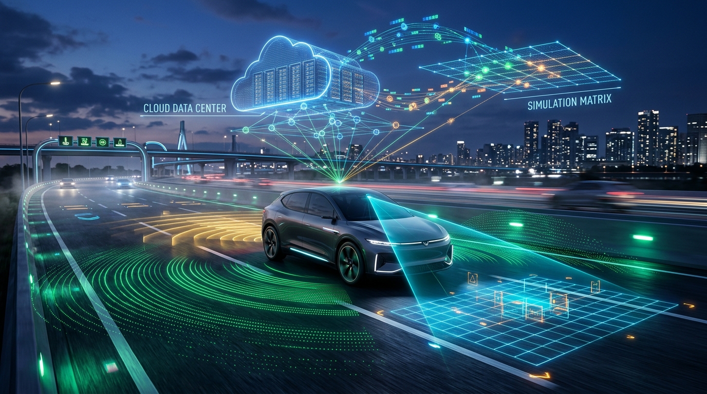
Building a production autonomous vehicle is far more than slapping an AI chip onto a dashboard. It requires a synchronized data factory spanning three specialized computers:
flowchart TD
    subgraph Computer1["Computer 1: Data Center AI Training (NVIDIA DGX)"]
        direction TB
        T1["Petabytes of Real Fleet Video & Synthetic Driving Logs"] --> T2["Cosmos Curate: Automatic Tagging & Corner-Case Retrieval"]
        T2 --> T3["Pre-Training Alpamayo Vision-World-Trajectory Models"]
    end
    style Computer1 fill:#0f172a,stroke:#00e5ff,stroke-width:2px,color:#ffffff
    style T1 fill:#0d2b45,stroke:#00e5ff,stroke-width:1px,color:#ffffff
    style T2 fill:#0d2b45,stroke:#00e5ff,stroke-width:1px,color:#ffffff
    style T3 fill:#0d2b45,stroke:#00e5ff,stroke-width:1px,color:#ffffff
flowchart TD
subgraph Computer2["Computer 2: Digital Twin Simulation (NVIDIA Omniverse on RTX PRO)"]
direction TB
M1["NuRec 3D Neural Scene Reconstruction from Real Drives"] --> M2["Cosmos Generative AI: Synthesizing Rare Rain & Glare Scenarios"]
M2 --> M3["AlpaSim Closed-Loop Software-in-the-Loop (SIL) Validation"]
end
style Computer2 fill:#0f172a,stroke:#818cf8,stroke-width:2px,color:#ffffff
style M1 fill:#1e1b4b,stroke:#818cf8,stroke-width:1px,color:#ffffff
style M2 fill:#1e1b4b,stroke:#818cf8,stroke-width:1px,color:#ffffff
style M3 fill:#1e1b4b,stroke:#818cf8,stroke-width:1px,color:#ffffffflowchart TD
subgraph Computer3["Computer 3: In-Vehicle Real-Time Execution (NVIDIA DRIVE AGX / Thor)"]
direction TB
V1["DRIVE Hyperion 360° Sensor Ingestion (12 Cams, 9 Radars, 1 LiDAR)"] --> V2["Real-Time Bird's-Eye-View (BEV) Transformer Spatial Fusion"]
V2 --> V3["ASIL-D Dual-Lockstep Safety Island & Direct Steer/Brake Actuation"]
end
style Computer3 fill:#0f172a,stroke:#10b981,stroke-width:2px,color:#ffffff
style V1 fill:#1a3d3c,stroke:#10b981,stroke-width:1px,color:#ffffff
style V2 fill:#0d2b45,stroke:#00e5ff,stroke-width:1px,color:#ffffff
style V3 fill:#0f382c,stroke:#10b981,stroke-width:1px,color:#ffffff- Training Computer (NVIDIA DGX): The supercomputer brain in the cloud where petabytes of real-world fleet data are filtered by Cosmos Curate, indexing rare edge cases (e.g., a mattress falling off a truck) and training multi-billion parameter foundation models.
- Simulation Computer (NVIDIA Omniverse on RTX PRO): The virtual proving ground where Omniverse NuRec reconstructs real routes into photorealistic digital twins, while Cosmos injects hazardous weather variations to stress-test driving policies across billions of virtual miles in AlpaSim.
- In-Vehicle Computer (NVIDIA DRIVE Thor & DRIVE Hyperion): The production-ready reference architecture integrating standardized 360° sensor suites (exterior cameras, radars, LiDARs, ultrasonics) and redundant compute into an ISO 26262 ASIL-D certified platform. Combined with NVIDIA Halos safety validation, it executes real-time neural perception and emergency fallback actuation in under 25 milliseconds.
3. Demystifying the 6 SAE Autonomy Levels
The Society of Automotive Engineers (SAE) defines six levels of driving automation (SAE J3016) based on who does what, when:
flowchart TD
    L0["Level 0: No Automation (Human Drives; Momentary Alerts)"] --> L1["Level 1: Driver Assist (Adaptive Cruise Control OR Lane Keeping)"]
    L1 --> L2["Level 2 / 2+: Partial Automation (Steering AND Speed; Driver Supervises)"]
    L2 --> L3["Level 3: Conditional Automation (Car Drives; Driver Takes Over on Alert)"]
    L3 --> L4["Level 4: High Automation (Full Autonomy in Geofenced ODD / Robotaxis)"]
    L4 --> L5["Level 5: Full Automation (Any Road, Any Weather, No Steering Wheel)"]

    style L0 fill:#1e293b,stroke:#ef4444,stroke-width:1px,color:#ffffff
    style L1 fill:#1e293b,stroke:#f59e0b,stroke-width:1px,color:#ffffff
    style L2 fill:#0d2b45,stroke:#00e5ff,stroke-width:1px,color:#ffffff
    style L3 fill:#1e1b4b,stroke:#818cf8,stroke-width:2px,color:#ffffff
    style L4 fill:#1a3d3c,stroke:#10b981,stroke-width:2px,color:#ffffff
    style L5 fill:#0f382c,stroke:#10b981,stroke-width:2px,color:#ffffff
SAE Autonomy Classification Matrix
| SAE Level | Autonomy Tier | Steering & Acceleration | Environmental Monitoring | Fallback Responsibility | Typical Commercial Example |
|---|---|---|---|---|---|
| Level 0 | No Automation | Human | Human | Human | Automatic Emergency Braking (AEB) |
| Level 1 | Driver Assistance | System OR Human | Human | Human | Basic Adaptive Cruise Control |
| Level 2 | Partial Automation | System | Human | Human (Eyes on road) | Highway Lane Centering + ACC |
| Level 2+ / 2++ | Expanded Automation | System | System / Human | Human (Hands-off, Eyes-on) | NVIDIA DRIVE AV Supervised Highway |
| Level 3 | Conditional Automation | System | System | Human on Request (10s buffer) | Traffic Jam Pilot on certified freeways |
| Level 4 | High Automation | System | System | System (Minimum Risk Maneuver) | Commercial Urban Robotaxis & Hub Fleets |
| Level 5 | Full Automation | System | System | System (No steering wheel) | Universal all-weather autonomous transport |
4. The Sensor Modality Matrix: Cameras, Radars, and LiDARs
No single sensor is sufficient for safety-critical autonomous mobility. Each modality brings distinct physical advantages:
flowchart TD
    subgraph SensorSuite["Multimodal 360° Sensor Ingestion Topology"]
        direction TB
        C1["1. Optical Cameras (400-700 nm)<br/>• Rich semantic RGB color, traffic signals & lane marking OCR<br/>• High angular resolution; vulnerable to glare and dense fog"]
        C1 --> R1["2. 77 GHz Millimeter-Wave Radar<br/>• Direct radial Doppler velocity measurement<br/>• Robust penetration through heavy rain, snow, mist & night darkness"]
        R1 --> L1["3. 3D Time-of-Flight LiDAR (905 / 1550 nm)<br/>• Millimeter-accurate 3D point clouds & geometric occupancy<br/>• Complete day/night lighting invariance"]
        L1 --> U1["4. Ultrasonic Transducers<br/>• Short-range proximity detection (< 3m) for tight parking maneuvers"]
        U1 --> F1["Centralized Multi-Sensor Kalman & BEV Transformer Fusion Engine"]
    end
    style SensorSuite fill:#0f172a,stroke:#00e5ff,stroke-width:2px,color:#ffffff
    style C1 fill:#0d2b45,stroke:#00e5ff,stroke-width:1px,color:#ffffff
    style R1 fill:#1e1b4b,stroke:#818cf8,stroke-width:1px,color:#ffffff
    style L1 fill:#1a3d3c,stroke:#10b981,stroke-width:1px,color:#ffffff
    style U1 fill:#1e293b,stroke:#f59e0b,stroke-width:1px,color:#ffffff
    style F1 fill:#0f382c,stroke:#10b981,stroke-width:2px,color:#ffffff
Sensor Physics Comparison
- Cameras (Optical $400 - 700\text{ nm}$): Highest resolution and lowest cost. Essential for reading traffic lights, road text, and lane markers. Vulnerable to sun glare, dirty lenses, and dense fog.
- Radar (Millimeter Wave $76 - 81\text{ GHz}$): Measures object range and direct radial velocity via the Doppler frequency shift. Unaffected by rain, snow, fog, or darkness. Lower angular resolution for fine object classification.
- LiDAR (Infrared Lasers $905\text{ nm} / 1550\text{ nm}$): Fires up to 2 million laser pulses per second, directly calculating photon time-of-flight to generate dense 3D geometric point clouds. Invariant to external lighting conditions.
5. Engineering Deep-Dive: Mathematical Formulations
To understand how multiple noisy sensor measurements are fused and how Operational Design Domains are evaluated, we review the formal mathematics.
Mathematical Formulation 1: Multi-Sensor Covariance Intersection & Fusion
When fusing independent observations $z_i$ from $N$ sensor modalities with measurement error covariance matrices $R_i$, the optimal Maximum Likelihood State Estimate $\hat{x}{\text{fused}}$ and its posterior covariance $P{\text{fused}}$ are computed as:
$$P_{\text{fused}} = \left( \sum_{i=1}^N R_i^{-1} \right)^{-1}$$
$$\hat{x}{\text{fused}} = P{\text{fused}} \left( \sum_{i=1}^N R_i^{-1} z_i \right)$$
Because $\sum R_i^{-1} > R_k^{-1}$ for any single sensor $k$, the fused uncertainty is strictly smaller than any individual sensor ($P_{\text{fused}} < R_k$). Even if a camera’s variance spikes ($R_{\text{cam}} \to \infty$) in blinding fog, radar and LiDAR keep $P_{\text{fused}}$ bounded.
Mathematical Formulation 2: Radar Doppler Radial Velocity Vector Resolution
A 77 GHz automotive radar measures the radial velocity $v_r$ of a moving target relative to the vehicle’s heading vector $\theta$:
$$v_r = \vec{v}_{\text{target}} \cdot \hat{r} = v_x \cos\theta + v_y \sin\theta$$
Where the Doppler frequency shift $\Delta f$ directly reveals velocity:
$$\Delta f = \frac{2 f_0 v_r}{c}$$
Providing instantaneous velocity measurements without requiring multi-frame optical tracking differentials.
Mathematical Formulation 3: Operational Design Domain (ODD) State Verification
A vehicle’s Operational Design Domain is defined as a bounded parameter space $\Omega_{\text{ODD}} \subset \mathbb{R}^D$ encompassing road types, weather conditions, and sensor uncertainties:
$$\mathcal{P}\left(\text{State} \in \Omega_{\text{ODD}} \mid \mathbf{Z}\right) = \prod_{k=1}^D \mathbb{I}\left( z_k \in [\text{min}_k, \text{max}k] \right) \ge \Gamma{\text{safety}}$$
If adverse weather causes $\mathcal{P} < \Gamma_{\text{safety}}$, the system immediately initiates a safe degradation transition (e.g., Level 4 Minimal Risk Maneuver).
6. Interactive Python Simulation
The zero-dependency Python script below simulates multi-sensor Kalman fusion under varying weather conditions (Clear Daylight, Heavy Rain & Fog, Blizzard) and arbitrates active SAE Autonomy Levels:
Click to expand runnable Python simulation script
#!/usr/bin/env python3
"""
Autonomous Vehicle Fundamentals & Multi-Sensor Fusion Simulator
================================================================
A standalone, zero-dependency Python simulation demonstrating:
1. Multimodal Sensor Modality Modeling (Camera, Radar, LiDAR).
2. Extended Kalman Filter (EKF) Multi-Sensor State Estimation under Adverse Weather.
3. SAE Autonomy Levels & Operational Design Domain (ODD) Boundary Evaluation.
"""

import math
import random
from typing import Dict, List, Tuple, Optional

# ============================================================================
# 1. SENSOR MODALITY MODELS & ADVERSE ENVIRONMENT PERTURBATIONS
# ============================================================================

class SensorObservation:
    def __init__(self, sensor_name: str, x: float, y: float, vx: float, vy: float, variance: float, valid: bool):
        self.sensor_name = sensor_name
        self.x = x
        self.y = y
        self.vx = vx
        self.vy = vy
        self.variance = variance
        self.valid = valid


class AutonomousVehicleSensors:
    def __init__(self, true_x: float, true_y: float, true_vx: float, true_vy: float):
        self.true_x = true_x
        self.true_y = true_y
        self.true_vx = true_vx
        self.true_vy = true_vy

    def sample_sensors(self, weather: str = "heavy_rain_fog") -> List[SensorObservation]:
        """Simulates raw sensor readings with realistic physics-based noise profiles."""
        obs = []

        if weather == "clear_daylight":
            cam_var, radar_var, lidar_var = 0.05, 0.40, 0.02
            cam_drop, radar_drop, lidar_drop = 0.0, 0.0, 0.0
        elif weather == "heavy_rain_fog":
            cam_var, radar_var, lidar_var = 1.80, 0.45, 0.35
            cam_drop, radar_drop, lidar_drop = 0.30, 0.02, 0.15
        else:  # dense_night_blizzard
            cam_var, radar_var, lidar_var = 4.50, 0.55, 1.20
            cam_drop, radar_drop, lidar_drop = 0.70, 0.05, 0.40

        # 1. Camera
        if random.random() > cam_drop:
            cx = self.true_x + random.gauss(0, math.sqrt(cam_var))
            cy = self.true_y + random.gauss(0, math.sqrt(cam_var))
            cvx = self.true_vx + random.gauss(0, math.sqrt(cam_var * 2.0))
            cvy = self.true_vy + random.gauss(0, math.sqrt(cam_var * 2.0))
            obs.append(SensorObservation("Camera (RGB)", cx, cy, cvx, cvy, cam_var, True))
        else:
            obs.append(SensorObservation("Camera (RGB)", 0.0, 0.0, 0.0, 0.0, 999.0, False))

        # 2. Radar
        if random.random() > radar_drop:
            rx = self.true_x + random.gauss(0, math.sqrt(radar_var))
            ry = self.true_y + random.gauss(0, math.sqrt(radar_var))
            rvx = self.true_vx + random.gauss(0, 0.08)
            rvy = self.true_vy + random.gauss(0, 0.08)
            obs.append(SensorObservation("Radar (77GHz Doppler)", rx, ry, rvx, rvy, radar_var, True))
        else:
            obs.append(SensorObservation("Radar (77GHz Doppler)", 0.0, 0.0, 0.0, 0.0, 999.0, False))

        # 3. LiDAR
        if random.random() > lidar_drop:
            lx = self.true_x + random.gauss(0, math.sqrt(lidar_var))
            ly = self.true_y + random.gauss(0, math.sqrt(lidar_var))
            lvx = self.true_vx + random.gauss(0, math.sqrt(lidar_var * 1.5))
            lvy = self.true_vy + random.gauss(0, math.sqrt(lidar_var * 1.5))
            obs.append(SensorObservation("LiDAR (3D Point Cloud)", lx, ly, lvx, lvy, lidar_var, True))
        else:
            obs.append(SensorObservation("LiDAR (3D Point Cloud)", 0.0, 0.0, 0.0, 0.0, 999.0, False))

        return obs


# ============================================================================
# 2. MULTI-SENSOR KALMAN FILTER FUSION ENGINE
# ============================================================================

class MultiSensorFusionEngine:
    def __init__(self):
        self.state = [0.0, 0.0, 0.0, 0.0]
        self.covariance = [1.0, 1.0, 1.0, 1.0]

    def fuse_observations(self, observations: List[SensorObservation]) -> Tuple[List[float], List[float]]:
        """Fuses asynchronous multimodal observations using optimal variance weighting."""
        valid_obs = [o for o in observations if o.valid]
        if not valid_obs:
            return self.state, self.covariance

        inv_vars_pos = [1.0 / o.variance for o in valid_obs]
        total_inv_pos = sum(inv_vars_pos)
        weights_pos = [iv / total_inv_pos for iv in inv_vars_pos]

        fused_x = sum(w * o.x for w, o in zip(weights_pos, valid_obs))
        fused_y = sum(w * o.y for w, o in zip(weights_pos, valid_obs))
        fused_var_pos = 1.0 / total_inv_pos

        inv_vars_vel = []
        for o in valid_obs:
            v_var = 0.02 if "Radar" in o.sensor_name else o.variance * 1.5
            inv_vars_vel.append(1.0 / v_var)
        total_inv_vel = sum(inv_vars_vel)
        weights_vel = [iv / total_inv_vel for iv in inv_vars_vel]

        fused_vx = sum(w * o.vx for w, o in zip(weights_vel, valid_obs))
        fused_vy = sum(w * o.vy for w, o in zip(weights_vel, valid_obs))
        fused_var_vel = 1.0 / total_inv_vel

        self.state = [fused_x, fused_y, fused_vx, fused_vy]
        self.covariance = [fused_var_pos, fused_var_pos, fused_var_vel, fused_var_vel]
        return self.state, self.covariance


# ============================================================================
# 3. SAE AUTONOMY LEVELS & OPERATIONAL DESIGN DOMAIN (ODD) ARBITRATOR
# ============================================================================

class OperationalDesignDomain:
    @staticmethod
    def evaluate_sae_level(weather: str, fused_pos_uncertainty: float, hd_map_confidence: float) -> Dict[str, str]:
        """Evaluates operational boundaries and matches the system to SAE Autonomy Levels."""
        if fused_pos_uncertainty < 0.10 and hd_map_confidence > 0.90 and weather == "clear_daylight":
            return {
                "active_level": "SAE Level 4 (High Automation)",
                "driver_role": "Passenger (Zero supervision required in geofenced ODD)",
                "fallback_mode": "Autonomous Minimum Risk Maneuver (Pull to Shoulder)",
                "odd_status": "✅ FULL ODD COMPLIANCE",
            }
        elif fused_pos_uncertainty < 0.35 and hd_map_confidence > 0.70:
            return {
                "active_level": "SAE Level 3 (Conditional Automation)",
                "driver_role": "Fallback Ready (Must resume control within 10s upon request)",
                "fallback_mode": "Driver Handover Request -> Controlled Deceleration",
                "odd_status": "⚠️ CONDITIONAL ODD (Weather / Vision degraded)",
            }
        elif fused_pos_uncertainty < 0.80:
            return {
                "active_level": "SAE Level 2+ (Expanded Supervised ADAS)",
                "driver_role": "Active Supervisor (Hands-on / Eyes-on-road mandatory)",
                "fallback_mode": "Immediate Driver Takeover & Audible Chime",
                "odd_status": "⚠️ RESTRICTED ODD (Driver actively steering)",
            }
        else:
            return {
                "active_level": "SAE Level 0 / 1 (Driver in Full Command)",
                "driver_role": "Active Driver (Emergency Braking Assist active only)",
                "fallback_mode": "Full Manual Control",
                "odd_status": "❌ OUTSIDE OPERATIONAL DESIGN DOMAIN",
            }


# ============================================================================
# 4. SIMULATION PIPELINE EXECUTION
# ============================================================================

def run_av_fundamentals_simulation():
    random.seed(42)
    print("=" * 85)
    print("AUTONOMOUS VEHICLE FUNDAMENTALS & MULTI-SENSOR FUSION BENCHMARK")
    print("=" * 85)

    true_target = {"x": 42.0, "y": 1.2, "vx": 22.0, "vy": 0.0}
    sensors = AutonomousVehicleSensors(true_target["x"], true_target["y"], true_target["vx"], true_target["vy"])
    fusion_engine = MultiSensorFusionEngine()

    print(f"\n[1] GROUND TRUTH OBSTACLE STATE:")
    print(f"  • Position: X={true_target['x']:.2f} m (Forward), Y={true_target['y']:.2f} m (Lateral)")
    print(f"  • Velocity: Vx={true_target['vx']:.2f} m/s ({true_target['vx']*3.6:.1f} km/h), Vy={true_target['vy']:.2f} m/s")

    test_weathers = ["clear_daylight", "heavy_rain_fog", "dense_night_blizzard"]

    for w_idx, weather in enumerate(test_weathers, 1):
        print("\n" + "-" * 85)
        print(f"[{w_idx}] SCENARIO EVALUATION: Weather = {weather.upper()}")
        print("-" * 85)

        raw_observations = sensors.sample_sensors(weather=weather)
        print(f"{'Sensor Modality':<25} | {'Obs X (m)':<10} | {'Obs Y (m)':<10} | {'Obs Vx (m/s)':<14} | {'Status'}")
        print("-" * 85)
        for o in raw_observations:
            if o.valid:
                print(f"{o.sensor_name:<25} | {o.x:>8.2f} m | {o.y:>8.2f} m | {o.vx:>10.2f} m/s  | ✅ ACTIVE (var={o.variance:.2f})")
            else:
                print(f"{o.sensor_name:<25} | {'--':>8}   | {'--':>8}   | {'--':>10}      | ❌ BLINDED / OCCLUDED")

        fused_state, fused_cov = fusion_engine.fuse_observations(raw_observations)
        pos_error = math.hypot(fused_state[0] - true_target["x"], fused_state[1] - true_target["y"])
        vel_error = math.hypot(fused_state[2] - true_target["vx"], fused_state[3] - true_target["vy"])

        print(f"\n  🎯 MULTI-SENSOR FUSED ESTIMATE:")
        print(f"     Position: X={fused_state[0]:.2f} m, Y={fused_state[1]:.2f} m (Position Error: {pos_error:.3f} m, Uncertainty: ±{math.sqrt(fused_cov[0]):.3f}m)")
        print(f"     Velocity: Vx={fused_state[2]:.2f} m/s ({fused_state[2]*3.6:.1f} km/h), Vy={fused_state[3]:.2f} m/s (Velocity Error: {vel_error:.3f} m/s)")

        hd_map_conf = 0.95 if weather == "clear_daylight" else (0.80 if weather == "heavy_rain_fog" else 0.50)
        odd_decision = OperationalDesignDomain.evaluate_sae_level(weather, fused_cov[0], hd_map_conf)

        print(f"\n  🛡️ ODD & SAE LEVEL ARBITRATION:")
        print(f"     • Operating Mode: {odd_decision['active_level']}")
        print(f"     • Driver Role:    {odd_decision['driver_role']}")
        print(f"     • Fallback Rule:  {odd_decision['fallback_mode']}")
        print(f"     • ODD Health:     {odd_decision['odd_status']}")

    print("=" * 85)


if __name__ == "__main__":
    run_av_fundamentals_simulation()
7. Conclusion: The Full Physical AI & Robotics Arc
Across our 9-part NVIDIA Physical AI & Robotics Ecosystem Series, we have journeyed through the entire Physical AI spectrum:
- The Data Factory & World Models (Part 1 & Part 2): Generating synthetic physical commonsense with NVIDIA Cosmos.
- Simulation & Digital Twins (Part 3, Part 4, Part 5): OpenUSD composition, RTX ray tracing, and PhysX 5 GPU-accelerated domain randomization.
- Embodied Foundation Models (Part 6): Humanoid sensorimotor intelligence via Project GR00T and diffusion action chunking.
- End-to-End Autonomous Vehicles (Part 7 & Part 9): 360° BEV transformer fusion, Alpamayo foundation models, SAE Level 0–5 autonomy tiers, and multimodal sensor fusion.
- Edge Silicon & Zero-Copy Reflexes (Part 8): Deploying foundation models on Jetson Thor with Isaac ROS NITROS for sub-50ms physical agility.
By unifying data centers, photorealistic physics simulations, and in-vehicle edge computing, autonomous vehicles and humanoid robots are transforming from futuristic research into real-world everyday intelligence.