
Part 9: The Evolutionary Arc of Computer Vision: From LeNet-5 and ResNet to ConvNeXt and 3D Video Models
How did computer vision evolve from reading bank check zip codes in 1998 to 3D video spatial physics in physical AI and robotics?
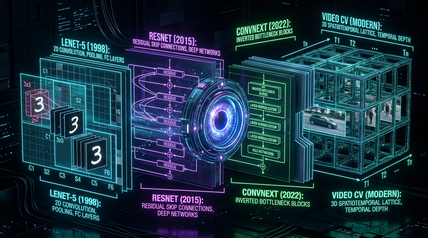
Series: Neural Architecture Evolution Series (From MLPs to Transformers) - Part 9
Series: ← Part 8: Generative Adversarial Networks (GANs): The Counterfeiter vs. Detective Minimax Game (Previous)
Prior Reading Material
Before exploring spatial convolutions and temporal video modeling, inspect these foundational deep-dives across our blog:
- Part 1: Demystifying Neural Networks — Biological neurons, perceptrons, MLPs, 2D CNNs, and standard Recurrent Neural Networks (RNNs).
- Part 4: Demystifying Activation Functions — Why neural networks require non-linear space warping (Sigmoid, ReLU, GELU, SwiGLU).
- Part 6: Why Deep Networks Die — Weight initialization (He/Xavier), LayerNorm/RMSNorm, and ResNet residual skip connections.
- Physical AI Models: Grounding Intelligence in Space, Physics, and Robotics — Spatial grounding, visual encoders, and robotic manipulation pipelines.
- The Architectural Spectrum of World Foundation Models — Renderers, state simulators, and action planners for spatial video generation.
1. The Story of the Sliding Flashlight & The 3D Film Reel
How does a machine look at a 2D grid of raw RGB pixels and instantly recognize a cat, a pedestrian, or a moving vehicle?
To understand how vision architectures evolved over three decades, imagine inspecting a giant dark painting using a specialized Sliding Flashlight:
-
LeNet-5 (1998) [The Sliding 2D Flashlight]:
- Yann LeCun introduced LeNet-5 to scan handwritten digits on bank checks.
- A tiny $5 \times 5$ flashlight grid (a Convolutional Filter) slides across an image pixel by pixel, multiplying pixel brightness by filter weights.
- Translation Invariance: Whether a handwritten
"3"appears in the top-left corner or bottom-right corner, the same flashlight detects its curved edges!
-
ResNet (2015) [The Deep Skyscraper Highways]:
- As networks stacked more layers to detect complex objects, signals vanished (Part 6).
- Kaiming He introduced Residual Skip Connections ($y = F(x) + x$), creating express elevator highways that allowed vision networks to scale from 16 layers (VGG) to 152+ layers (ResNet)!
-
ConvNeXt (2022) [The Modernized CNN Counterattack]:
- When Vision Transformers (ViT) threatened to replace CNNs, Meta AI introduced ConvNeXt.
- By adopting Transformer design choices—large $7 \times 7$ depthwise kernels, inverted bottleneck blocks, LayerNorm, and GELU activations—ConvNeXt proved that pure convolutional networks can match or exceed Vision Transformers while being faster and using far less memory!
-
3D Video Models (Modern) [The 3D Film Reel Cube]:
- Single 2D images cannot capture motion, speed, or causality. A car stopped at a red light looks identical to a car speeding through an intersection in a static frame!
- 3D Video Convolutions ($3D\text{-CNNs}$) extend the flashlight into a 3D spatiotemporal cube ($K_T \times K_H \times K_W$), scanning across space (height and width) and time (frames) simultaneously!
2. Visualizing Vision Architecture Layouts
The following vertical workflow diagrams contrast how spatial and temporal features are processed across different computer vision paradigms:
Case 1: ResNet Residual Block vs. ConvNeXt Modernized Inverted Bottleneck
Path 1: Standard ResNet Residual Block (2015)
flowchart TD
    R_IN["1. Input Feature Map X"]
    R_CONV1["2. 1x1 Conv (Bottleneck Compress) + BatchNorm + ReLU"]
    R_CONV2["3. 3x3 Spatial Conv + BatchNorm + ReLU"]
    R_CONV3["4. 1x1 Conv (Expand) + BatchNorm"]
    R_ADD["5. Identity Addition (+ X) + Final ReLU"]

    R_IN --> R_CONV1 --> R_CONV2 --> R_CONV3 --> R_ADD

    style R_IN fill:#0f172a,stroke:#38bdf8,stroke-width:2px,color:#ffffff
    style R_CONV1 fill:#1e1b4b,stroke:#818cf8,stroke-width:2px,color:#ffffff
    style R_CONV2 fill:#0d2b45,stroke:#00e5ff,stroke-width:2px,color:#ffffff
    style R_CONV3 fill:#1e1b4b,stroke:#818cf8,stroke-width:2px,color:#ffffff
    style R_ADD fill:#14532d,stroke:#22c55e,stroke-width:2px,color:#ffffff
Path 2: ConvNeXt Inverted Bottleneck Block (2022)
flowchart TD
    C_IN["1. Input Feature Map X"]
    C_DW["2. 7x7 Depthwise Conv (Large Spatial Receptive Field)"]
    C_LN["3. LayerNorm (Channel Normalization)"]
    C_PW1["4. 1x1 Pointwise Conv (Expand 4x Channels) + GELU"]
    C_PW2["5. 1x1 Pointwise Conv (Compress back to original channels)"]
    C_ADD["6. Identity Addition (+ X)"]

    C_IN --> C_DW --> C_LN --> C_PW1 --> C_PW2 --> C_ADD

    style C_IN fill:#0f172a,stroke:#38bdf8,stroke-width:2px,color:#ffffff
    style C_DW fill:#1e1b4b,stroke:#818cf8,stroke-width:2px,color:#ffffff
    style C_LN fill:#581c87,stroke:#c084fc,stroke-width:2px,color:#ffffff
    style C_PW1 fill:#0d2b45,stroke:#00e5ff,stroke-width:2px,color:#ffffff
    style C_PW2 fill:#0d2b45,stroke:#00e5ff,stroke-width:2px,color:#ffffff
    style C_ADD fill:#14532d,stroke:#22c55e,stroke-width:2px,color:#ffffff
Case 2: 3D Video Spatiotemporal Convolution Pipeline
flowchart TD
    VIDEO_IN["1. Input Video Clip (T Frames x H Height x W Width x C Channels)"]
    CONV3D["2. 3D Spatiotemporal Convolution Kernel (K_T x K_H x K_W)<br/>Scans across spatial pixels and consecutive temporal frames simultaneously"]
    FEAT3D["3. 3D Feature Map (Motion Trajectories + Spatial Geometry)"]
    POOL3D["4. 3D Global Spatiotemporal Pooling"]
    ACTION_OUT["5. Video Classification / Action Recognition Output"]

    VIDEO_IN --> CONV3D --> FEAT3D --> POOL3D --> ACTION_OUT

    style VIDEO_IN fill:#0f172a,stroke:#38bdf8,stroke-width:2px,color:#ffffff
    style CONV3D fill:#1e1b4b,stroke:#818cf8,stroke-width:2px,color:#ffffff
    style FEAT3D fill:#0d2b45,stroke:#00e5ff,stroke-width:2px,color:#ffffff
    style POOL3D fill:#581c87,stroke:#c084fc,stroke-width:2px,color:#ffffff
    style ACTION_OUT fill:#14532d,stroke:#22c55e,stroke-width:2px,color:#ffffff
3. Engineering Deep-Dive: Mathematical Formulations
Math in 1 Sentence: 2D Convolutions slide spatial weight matrices over pixels ($(I * K)(i, j)$), ConvNeXt decouples spatial filtering from channel mixing via Depthwise Separable Convolutions, and 3D Convolutions extend spatial kernels into time ($(V * K)(t, i, j)$) to extract motion dynamics.
1. 2D Spatial Convolution Equation
For an input image patch $I$ and a 2D filter kernel $K$ of size $k_h \times k_w$:
$$(I * K)(i, j) = \sum_{m=-a}^a \sum_{n=-b}^b I(i-m, j-n) \cdot K(m, n)$$
Where $a = \frac{k_h - 1}{2}$ and $b = \frac{k_w - 1}{2}$.
For multi-channel feature maps ($C_{\mathrm{in}} \to C_{\mathrm{out}}$), total floating point operations (FLOPs) scale as:
$$\text{FLOPs (2D Conv)} = 2 \cdot H \cdot W \cdot C_{\text{in}} \cdot C_{\text{out}} \cdot K_h \cdot K_w$$
2. Depthwise Separable Convolutions (ConvNeXt Efficiency)
Standard 2D convolution performs spatial filtering and channel mixing simultaneously, leading to high FLOPs. Depthwise Separable Convolutions decouple these operations into two steps:
- Depthwise Convolution (Spatial Filtering per Channel): Applies a single $K_h \times K_w$ kernel per input channel independently:
$$\text{FLOPs (Depthwise)} = 2 \cdot H \cdot W \cdot C_{\text{in}} \cdot K_h \cdot K_w$$
- Pointwise Convolution (Channel Mixing): Applies a $1 \times 1$ kernel to mix cross-channel representations:
$$\text{FLOPs (Pointwise)} = 2 \cdot H \cdot W \cdot C_{\text{in}} \cdot C_{\text{out}}$$
Total FLOPs reduction compared to standard convolution:
$$\text{Efficiency Ratio} = \frac{\text{FLOPs (Depthwise)} + \text{FLOPs (Pointwise)}}{\text{FLOPs (Standard 2D)}} = \frac{1}{C_{\text{out}}} + \frac{1}{K_h \cdot K_w}$$
Using a $7 \times 7$ ConvNeXt depthwise kernel cuts spatial calculation FLOPs by over 85%!
3. 3D Spatiotemporal Video Convolution Equation
When processing video clips (sequence of $T$ consecutive frames), 3D convolution slides a 3D kernel $K \in \mathbb{R}^{K_T \times K_H \times K_W}$ across time $t$ and space $(i, j)$:
$$(V * K)(t, i, j) = \sum_{p=-c}^c \sum_{m=-a}^a \sum_{n=-b}^b V(t-p, i-m, j-n) \cdot K(p, m, n)$$
Where $K_T$ captures frame-to-frame motion velocity and temporal causality essential for Physical AI and Autonomous Systems.
4. Engineering Comparison: Computer Vision Paradigms
| Feature | LeNet-5 / AlexNet (Classic) | ResNet-50 (Residual Benchmark) | ConvNeXt-Huge (Modernized CNN) | 3D Video CNNs (I3D / SlowFast) |
|---|---|---|---|---|
| Spatial Kernel Strategy | $5 \times 5$ & $11 \times 11$ Standard Convolutions | $3 \times 3$ Bottleneck Convolutions | $7 \times 7$ Depthwise Separable Convolutions | $3 \times 3 \times 3$ 3D Spatiotemporal Convolutions |
| Normalization & Activations | BatchNorm / ReLU | BatchNorm / ReLU | LayerNorm / GELU (Transformer-style) | BatchNorm3D / LayerNorm |
| Receptive Field Growth | Small local receptive fields | Medium receptive fields | Large global receptive fields | Spatiotemporal 3D volume |
| FLOPs Efficiency | High FLOPs per parameter | Balanced | Extremely High (85%+ FLOPs reduction) | High compute demand (temporal scaling) |
| Primary Target Adoption | Digit recognition, early ImageNet | Image classification, object detection | Modern vision backbones, Segment Anything (SAM) | Video action recognition, autonomous driving, World Models |
5. Interactive Python Simulation: 2D vs. ConvNeXt FLOPs & 2D Kernel Convolution
The following zero-dependency Python script computes exact FLOPs and parameter savings for ConvNeXt depthwise separable convolutions and simulates a 2D spatial convolution operation:
Click to expand runnable Python simulation script
#!/usr/bin/env python3
"""
Evolutionary Arc of Computer Vision Simulation: 2D Conv vs Depthwise Conv (ConvNeXt) vs 3D Video Conv

Demonstrates:
1. Pure Python standard library implementation of 2D spatial convolution and 3D spatiotemporal video convolution.
2. Parameter count and FLOPs comparison across vision architectures (LeNet-5, ResNet-50, ConvNeXt, 3D CNNs).
3. Demonstration of Depthwise Separable Convolution computational savings.
"""

import math
import random

def calc_2d_conv_flops(h_in, w_in, c_in, c_out, k_h, k_w):
    """Calculates FLOPs for standard 2D Convolution: 2 * H * W * C_in * C_out * K_h * K_w"""
    return 2 * h_in * w_in * c_in * c_out * k_h * k_w

def calc_depthwise_separable_conv_flops(h_in, w_in, c_in, c_out, k_h, k_w):
    """Calculates FLOPs for ConvNeXt Depthwise Separable Conv: Depthwise + Pointwise (1x1)"""
    dw_flops = 2 * h_in * w_in * c_in * k_h * k_w
    pw_flops = 2 * h_in * w_in * c_in * c_out * 1 * 1
    return dw_flops + pw_flops

def calc_3d_video_conv_flops(t_in, h_in, w_in, c_in, c_out, k_t, k_h, k_w):
    """Calculates FLOPs for 3D Video Convolution: 2 * T * H * W * C_in * C_out * K_t * K_h * K_w"""
    return 2 * t_in * h_in * w_in * c_in * c_out * k_t * k_h * k_w

def run_vision_evolution_sim():
    print("=" * 85)
    print("1. COMPUTER VISION ARCHITECTURE FLOPs & PARAMETER COMPUTATIONAL BENCHMARK")
    print("=" * 85)

    h_in, w_in = 56, 56
    c_in, c_out = 256, 256

    print(f"Feature Map Specification: Resolution={h_in}x{w_in}, Channels In={c_in}, Channels Out={c_out}\n")

    std_flops = calc_2d_conv_flops(h_in, w_in, c_in, c_out, 3, 3)
    std_params = c_in * c_out * 3 * 3

    dw_flops = calc_depthwise_separable_conv_flops(h_in, w_in, c_in, c_out, 7, 7)
    dw_params = (c_in * 7 * 7) + (c_in * c_out * 1 * 1)

    t_frames = 16
    video_flops = calc_3d_video_conv_flops(t_frames, h_in, w_in, c_in, c_out, 3, 3, 3)
    video_params = c_in * c_out * 3 * 3 * 3

    print(f"{'Architecture Paradigm':<42} | {'Params':<12} | {'GFLOPs':<10} | {'Efficiency Impact':<20}")
    print("-" * 85)
    print(f"{'Standard 2D Conv (ResNet 3x3)':<42} | {std_params/1e6:6.2f} M    | {std_flops/1e9:6.2f} G   | Baseline")
    print(f"{'Depthwise Separable Conv (ConvNeXt 7x7)':<42} | {dw_params/1e6:6.2f} M    | {dw_flops/1e9:6.2f} G   | {(1 - dw_flops/std_flops)*100:5.1f}% FLOPs Reduction")
    print(f"{'3D Video Conv (16 Frames, 3x3x3)':<42} | {video_params/1e6:6.2f} M    | {video_flops/1e9:6.2f} G   | {video_flops/std_flops:5.1f}x Temporal Expansion")

    print("\n")
    print("=" * 85)
    print("2. PURE PYTHON 2D SLIDING KERNEL CONVOLUTION SIMULATION (LeNet / ResNet)")
    print("=" * 85)

    random.seed(42)
    image_5x5 = [
        [1, 2, 0, 1, 3],
        [0, 1, 3, 2, 0],
        [2, 0, 1, 1, 2],
        [1, 3, 2, 0, 1],
        [0, 1, 0, 2, 3]
    ]

    kernel_3x3 = [
        [-1, -1, -1],
        [-1,  8, -1],
        [-1, -1, -1]
    ]

    output_3x3 = []
    for r in range(3):
        row = []
        for c in range(3):
            val = 0
            for kr in range(3):
                for kc in range(3):
                    val += image_5x5[r + kr][c + kc] * kernel_3x3[kr][kc]
            row.append(val)
        output_3x3.append(row)

    print("Input 5x5 Image Patch:")
    for row in image_5x5:
        print("  ", row)

    print("\nApplied 3x3 Edge Detection Kernel:")
    for row in kernel_3x3:
        print("  ", row)

    print("\nFeature Map Output 3x3 (Convolved Spatial Features):")
    for row in output_3x3:
        print("  ", row)

if __name__ == "__main__":
    run_vision_evolution_sim()